Taking Moshi Apart: A Conversation About Every Piece
A constructed dialogue between two people who work on voice systems from different ends. Ana builds speech language models. Ravi ships production voice agents on cascaded stacks. Every number and claim below is from the Moshi technical report or the primary source cited at the end; the conversation is a device, the facts are not.
Why the paper mattered at all
Ravi: Before we go component by component, I want to name the thing I actually felt when the demo went up in July 2024. I’ve shipped voice agents for three years. My users describe the experience the same way every time: it’s like a walkie-talkie. You talk, you stop, you wait, it talks. And when you try to cut in — “no, I meant the other Tuesday” — either it plows on deaf, or it hard-stops mid-syllable and you both restart into that half-second of mutual apology that never happens between two humans on a phone call.
Ana: And your instinct is that it’s a speed problem.
Ravi: That was my instinct for two years. It isn’t. I could make every stage
instant and the rhythm would survive, because the rhythm is in the control flow,
not the latency. Somewhere in my system there’s a boolean — call it
user_is_speaking — and every downstream behaviour is a consequence of when that
boolean flips.
while True:
    audio = mic.read_until_silence(threshold_ms=700)  # <-- the fatal hyperparameter
    text  = asr(audio)                                # paralinguistics deleted here
    reply = llm(history + [text])                     # waits for the full transcript
    speaker.play(tts(reply))                          # waits for the full reply
    # Nothing here can start before the line above it finishes. And for the whole
    # duration of that last line, the microphone is not being modelled at all.
Ana: That 700 is the number I’d point at. There’s no good value for it. Short enough not to interrupt a thinking pause, long enough not to trigger on a mid-sentence breath — those two constraints don’t have a common solution, because whether a silence means “I’m done” depends on the content of what came before it. You’re asking a threshold to do semantics.
Ravi: So what does Moshi do instead?
Ana: It deletes the question. Moshi never decides whether to speak. Every 80 milliseconds it emits a frame of audio for its own voice, unconditionally, forever. When it has nothing to say, those tokens decode to what the paper calls “natural silence” — a near-silent waveform. Not a reserved special value, not an absence of output. Just what the model predicts when it isn’t speaking.
Ravi: Silence becomes a thing you generate.
Ana: Silence becomes a thing you generate, and once it is, every turn-taking decision collapses into next-token prediction. Whether to start. Whether to keep going while the user is talking. Whether to drop a “yeah” in without taking the floor. All of it learned from data, under the same loss as everything else.
while True:
    user_frame = mimi.encode(mic.read(80_ms))     # 8 tokens, always, speech or not
    z = temporal_transformer(history)             # one pass per 80ms frame
    my_frame = depth_transformer(z, user_frame)   # text + 8 tokens for my own voice
    speaker.play(mimi.decode(my_frame.audio))     # silence is a decoded waveform
    history.append(my_frame + user_frame)

    # Notice what's NOT here: no VAD, no endpointing, no turn variable, no
    # interruption handler. There is no branch where a turn could be taken.
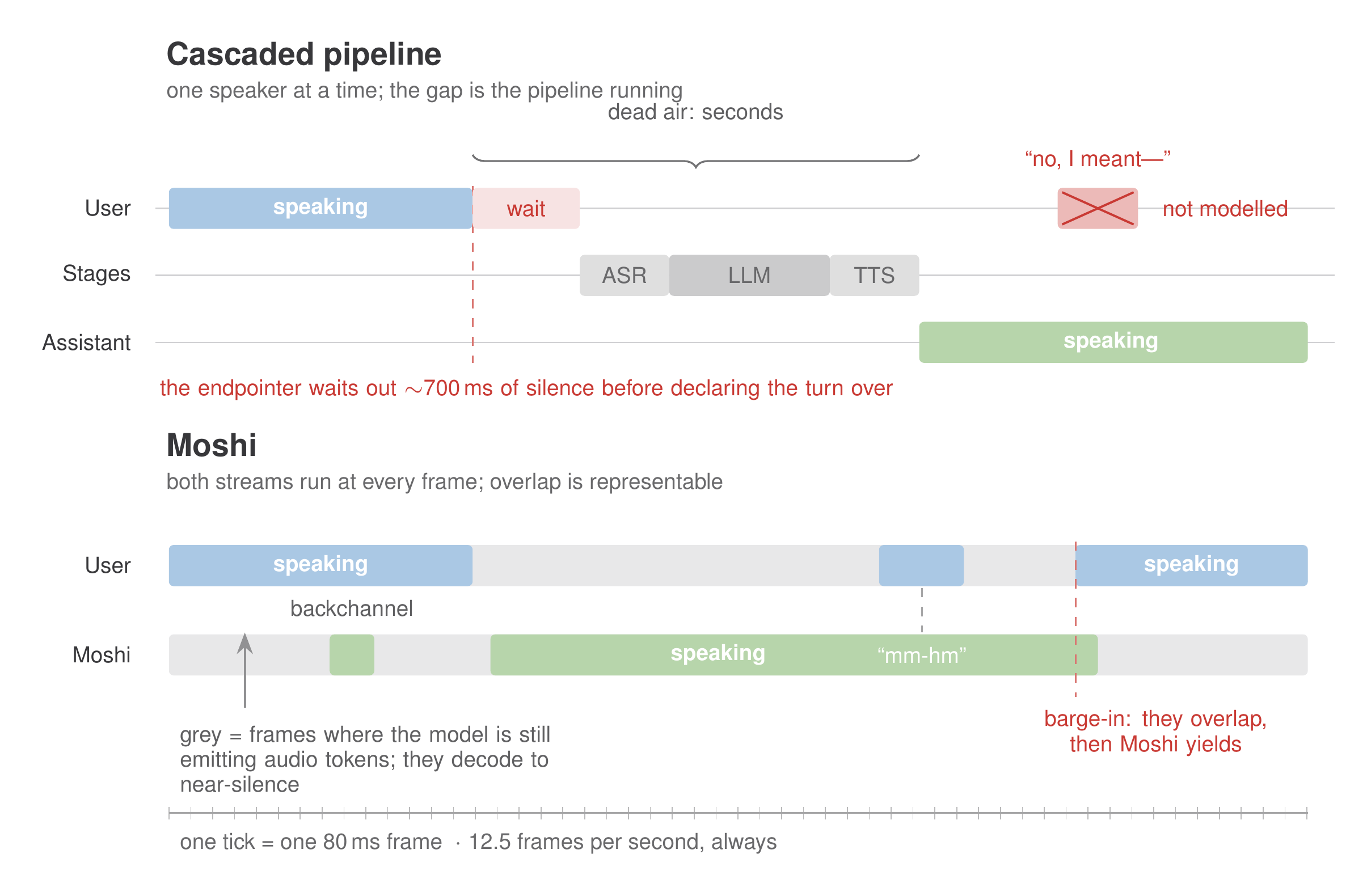
Figure 1 — A cascade partitions the conversation; Moshi doesn’t.
Ravi: Fine. But that reframe costs something, and I want to know what. Walk me down the stack.
Ana: Every component in the paper is what you have to build to afford a constant tick. Let’s start at the bottom, which is the part nobody writes about.
Helium: the backbone nobody talks about
Ravi: The text model. Kyutai trained it themselves — 7B, from scratch, 2.1 trillion tokens of public English.
Ana: Architecturally it’s boring on purpose. RMS normalisation at the input of the attention blocks, the feed-forward blocks, and the output linear layer. Rotary position embeddings. A 4,096-token context. FlashAttention. Gated linear units with SiLU as the gate. A 32,000-entry SentencePiece unigram tokenizer, English- targeted, with numbers split into individual digits and byte-backoff so nothing is lost.
Ravi: All standard. So why build it?
Ana: Two reasons, and the second one is the interesting one. The first is control over the tokenizer and the training mix, because everything else gets grafted onto this and the graft is invasive. The second is that they wanted the option to keep training on text after the audio training started. You can’t do that cleanly with a model whose data pipeline you don’t own.
Ravi: Say more about that, because it sounds like a footnote.
Ana: It’s the opposite of a footnote. During Moshi’s audio pre-training, half the batches are text-only, drawn from Helium’s original dataset, with a separate optimizer state so the two update streams stay balanced. They also multiply the learning rate on the text embedding and text output layer by 0.75 when operating on the text stream of an audio batch, and they halve the loss weight on padding tokens because padding dominates. Ablate the text batches away and spoken question answering drops across the board — Web Questions 26.6 to 23.2, Trivia QA 22.8 to 18.3.
Ravi: So warm-starting from a text model isn’t enough.
Ana: Warm-starting is not enough. That’s the transferable lesson and it’s cheap to state: a text model dropped into audio training forgets, and the fix is to keep reminding it, continuously, for a million steps.
Ravi: What about the data pipeline? I always skip those sections.
Ana: Don’t, this one has a reusable idea. 12.5% of the corpus is curated — Wikipedia across five different dumps rather than five passes over one, plus Wikibooks, Wikisource, Wikinews, StackExchange, and a scientific-article collection. The other 87.5% is CommonCrawl from ten specific crawls, filtered in three stages. Line-level deduplication inside each shard using an FNV-1a hash and a Bloom filter, to kill navigation boilerplate. Then a fastText classifier trained on duplicates versus non-duplicates for fuzzy dedup, removing blocks of at least three consecutive lines. Then language ID at the document level with a 0.85 threshold.
Ravi: And quality filtering?
Ana: This is the bit I’d steal. Rather than one “is this high quality” classifier, they train a nine-category fastText classifier where the classes are their high-quality sources — Wikipedia, Wikibooks, StackExchange split into STEM and humanities, and so on. It runs at line level, and the document score is a length-weighted average of line scores. So you’re not just measuring similarity to good text, you’re getting a domain profile you can filter on.
Ravi: What’s the result?
Ana: MMLU 54.3, competitive with open-weights models trained on similar compute budgets.
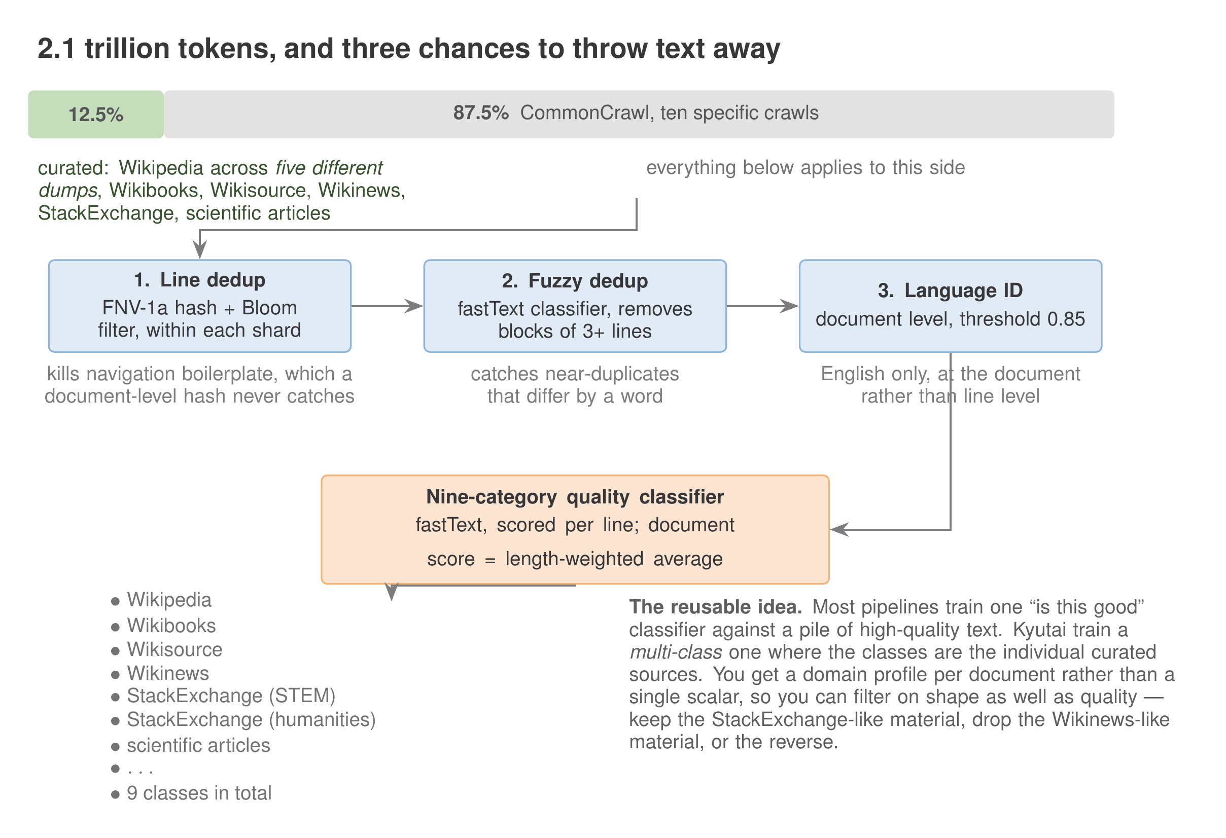
Figure 2 — Three chances to throw text away, and a classifier worth stealing. Which brings me to the “what next” for this component, and it’s a slightly deflating answer: almost nobody should do this now. If you’re building a speech model in 2026 you graft onto an existing strong text model. The reason Kyutai did it in 2024 was that the good open models had tokenizers and data mixes they couldn’t control.
Ravi: But then you inherit the graft problem without owning the pipeline.
Ana: Right, and that’s the live question. How do you keep a frontier text model’s knowledge through audio training when you can’t reconstruct its text corpus to interleave? The separate-optimizer-state trick still applies. The matched data doesn’t.
Mimi, part one: the frame rate is the latency budget
Ravi: The codec. Why couldn’t they use EnCodec?
Ana: Arithmetic. EnCodec and SoundStream run at 50 to 75 Hz. SpeechTokenizer runs at 50. Generating one frame of audio in Moshi costs a full forward pass through a 7B transformer, so the codec’s frame rate is the model’s inference rate. At 75 Hz you’re asking a 7B model to run seventy-five times a second.
Ravi: And text?
Ana: English text is roughly three to four tokens per second. That gap — two orders of magnitude between the natural rate of speech tokens and the natural rate of text tokens — is the central inefficiency of the whole field.
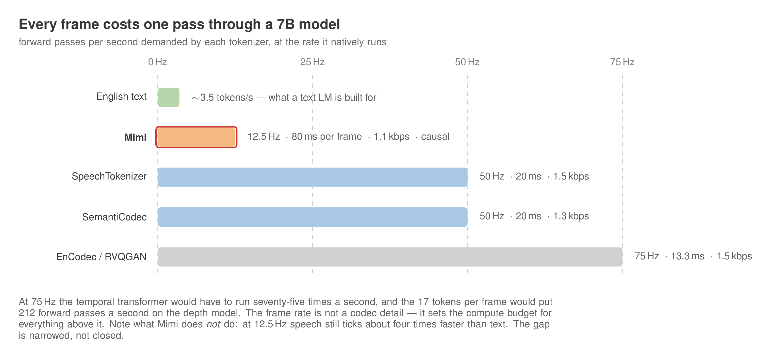
Figure 3 — The frame rate is not a codec detail; it is the compute budget.
Ravi: So Mimi closes it.
Ana: Mimi runs at 12.5 Hz. Concretely: a SeaNet autoencoder, four convolutional blocks with strides 4, 5, 6 and 8, plus a final 1D convolution with stride 2. That takes 24 kHz audio down to 12.5 frames per second at dimension 512. The decoder is symmetric with transposed convolutions. Every convolution is causal, so both encoding and decoding stream: hand it 80 milliseconds of audio, get one latent step out; hand it one latent step, get 80 milliseconds of audio back.
Ravi: 80 milliseconds is then a hard floor on response time.
Ana: A hard floor, non-negotiable, and it’s exactly half of Moshi’s 160 ms theoretical latency. The other 80 comes from the acoustic delay, which we’ll get to.
Ravi: What does that aggressive downsampling cost?
Ana: Capacity, which they buy back with Transformers in the bottleneck — one right before the quantizer and one right after. Eight layers, eight heads, model dimension 512, MLP dimension 2048, RoPE, GELU, LayerScale initialised at 0.01 for stability. Both are causally masked with a finite context of 250 frames, which is 20 seconds. So the codec preserves streaming end to end.
Ravi: Ablation says they help?
Ana: Both help perceived quality. And the encoder-side one helps a second thing that turns out to matter more, which is distillation — hold that thought.
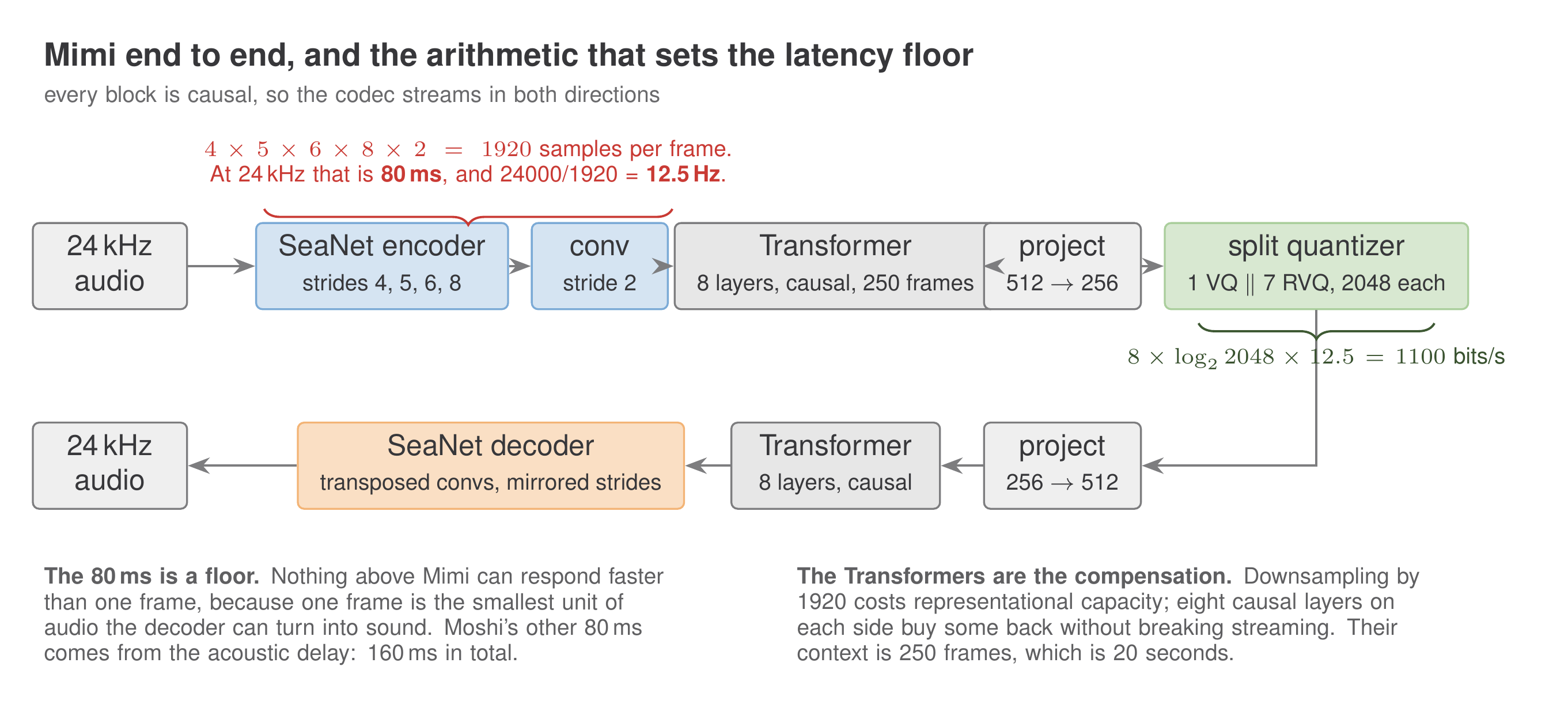
Figure 4 — Where the 80 milliseconds comes from.
Ravi: What about the quantizer configuration?
Ana: Eight quantizers, 2,048 entries each, which at 12.5 Hz is 1.1 kbps. The latent is 512-dimensional but they project down to 256 before quantizing and back up to 512 before the decoder. Quantizer dropout for bitrate scalability, following SoundStream. And one unusual choice: during training they only apply quantization 50% of the time, on a per-sequence basis, passing unquantized embeddings straight to the decoder the rest of the time.
Ravi: That’s different from the standard trick.
Ana: It’s a variant of an observation from the RVQGAN paper, but where they passed fully-quantized embeddings, Kyutai pass unquantized ones. It significantly improves objective quality, and — their words — the gain gets more significant as the bitrate drops, which they call counter-intuitive.
Ravi: So what’s the “what next” here?
Ana: 12.5 Hz became the target. It’s the number people design toward now, and there’s a live push lower — you’ll see codecs at 6.25 Hz and below, trading reconstruction for sequence length. But there’s a more interesting fork. The whole reason we’re counting frame rates is that we committed to discrete tokens and autoregressive decoding. If your output head is a flow-matching or diffusion head over continuous latents, the frame-rate arithmetic changes shape entirely. I don’t think that argument is settled.
Mimi, part two: the split RVQ, which is the best small idea in the paper
Ravi: Semantic versus acoustic tokens. Explain why those are two different things, because I’ve never understood why it isn’t just one tokenizer.
Ana: It’s historical, and the history is the explanation. Two research lineages arrived at speech tokens with opposite goals. Self-supervised speech encoders — wav2vec 2.0, HuBERT, WavLM — were built to produce features for recognition, so they were trained to throw away speaker identity, room acoustics, and prosody, keeping what distinguishes “beg” from “bag”. Neural codecs were built to compress, so they keep everything the ear notices and care nothing for linguistic structure.
Ravi: And you need both.
Ana: AudioLM established that you need both. Acoustic tokens alone don’t generate intelligible speech without text conditioning. Semantic tokens alone can’t be decoded into good audio. AudioLM’s answer was two separate tokenizers and a coarse-to-fine cascade: generate all the semantic tokens, then condition on them to generate the acoustic ones.
Ravi: Which is dead for real time.
Ana: Doubly dead. The semantic encoders are non-causal, so they can’t run online at all, and running two encoders is a compute burden you can’t afford at 12.5 Hz. So Mimi follows SpeechTokenizer: distil the semantic information into the codec’s own quantizer rather than running a second encoder.
Ravi: Distil from what?
Ana: WavLM. And there’s a mismatch to fix — WavLM takes 16 kHz and emits 1024-dimensional embeddings at 50 Hz; Mimi takes 24 kHz and emits 512 dimensions at 12.5 Hz. So during training they downsample the waveform to 16 kHz, run WavLM, and average-pool with stride 4 and kernel 8. The loss is a cosine distance between those embeddings and a linear projection of the first quantizer’s output.
Ravi: Kernel wider than stride. That pooling is looking into the future.
Ana: It is, and the paper says it was critical for performance that the pooling be non-causal. Which sounds like it should break streaming, and doesn’t, for a reason worth internalising: the teacher only exists at training time. WavLM never runs at inference. You can distil a bidirectional model into a causal one and keep the causality, because what you ship is the student.
Ravi: Okay. So where’s the problem?
Ana: The distillation fights the reconstruction, structurally. In a standard RVQ, quantizer 2 encodes the residual of quantizer 1, quantizer 3 encodes the residual of that, and so on. If you force quantizer 1 to be phonetic, you have changed what the residual is. Quantizers 2 through 8 now have to reconstruct audio starting from a sketch that was optimised to discard speaker identity and prosody.
Ravi: Show me it in the numbers.
Ana: Without distillation, phonetic discriminability — ABX error rate, lower is better — sits at 23.3%, which is useless for language modelling, while perceived quality on MUSHRA is 65.9. Turn distillation on: ABX drops to 6.5%, and MUSHRA falls to 57.8. You bought semantics with audio quality.
Ravi: And the fix?
Ana: Stop making it a residual. Instead of one 8-level RVQ, run a plain single-level VQ for semantics in parallel with a 7-level RVQ for acoustics, and sum their outputs before the decoder.
# Before: acoustics must reconstruct from what the semantic layer left behind.
z = encoder(x)
for q in quantizers[0:8]:
    code, z = q(z)                    # z is now the residual  <-- the conflict
    codes.append(code)

# After: two independent paths, summed. Nothing is anyone's leftovers.
z = encoder(x)
sem_code, sem_z = semantic_vq(z)      # distilled toward WavLM
aco_codes, aco_z = acoustic_rvq(z)    # 7 levels, sees the full z, not a residual
y = decoder(sem_z + aco_z)            # both paths reconstruct
Both paths still contribute to reconstruction. But the acoustic path no longer has to work from the semantic path’s leftovers. ABX degrades slightly to 8.1%; MUSHRA recovers to 64.0.
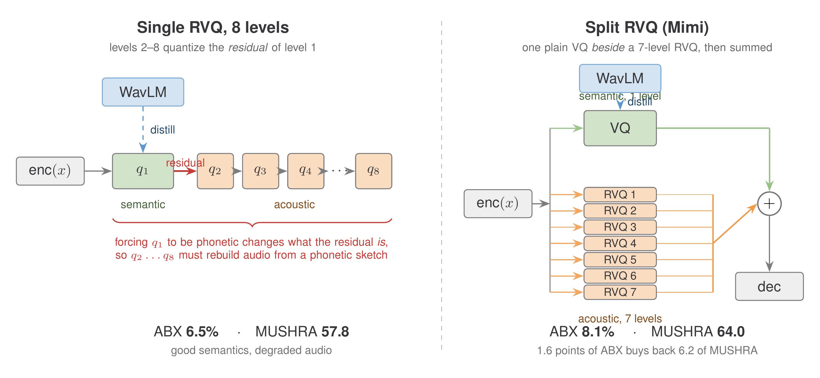
Figure 5 — Semantics and audio quality stop competing once they stop sharing a residual.
Ravi: 1.6 points of ABX for 6.2 of MUSHRA. That’s a good trade.
Ana: And it generalises past this paper, which is why I like it. Any time you distil an auxiliary objective into level one of a residual stack, you have created this conflict, whether or not you noticed. The fix is a shape change, not a hyperparameter.
Ravi: What’s the open question?
Ana: Whether semantic-versus-acoustic is even the right factorisation. It’s inherited from two accidents of research history, not derived from anything about speech. There are codecs now factorising along other axes — content, timbre, prosody as separate streams — and honestly nobody has shown which decomposition a language model actually wants. Mimi answered “how do I stop these two fighting”, not “are these the right two”.
Mimi, part three: the losses, and a broken instrument
Ravi: One more Mimi thing, because you flagged it earlier.
Ana: The loss ablation, which most labs would have buried. Neural codecs are normally trained with a mix of reconstruction losses — multi-scale mel-spectrogram — and adversarial losses, following EnCodec. Kyutai tried dropping the reconstruction losses entirely and keeping only the discriminator and feature- matching terms.
Ravi: And?
Ana: VisQOL, a standard objective similarity metric, collapsed from 2.82 to 1.84. Human MUSHRA raters went from 58.8 to 81.0.
Ravi: Those point in opposite directions.
Ana: They point in opposite directions and Kyutai shipped the adversarial-only version. Which means the reported VisQOL for the model they released is worse than the variant they rejected, and they put both in the table and said so.
Ravi: For context, where does that leave Mimi against other codecs?
Ana: At comparable bitrates: RVQGAN gets 31.3 MUSHRA at 1.5 kbps and 75 Hz. SpeechTokenizer 45.1 at 1.5 kbps and 50 Hz. SemantiCodec 64.8 at 1.3 kbps and 50 Hz. Mimi gets 81.0 at 1.1 kbps and 12.5 Hz — and unlike RVQGAN and SemantiCodec, it’s causal.
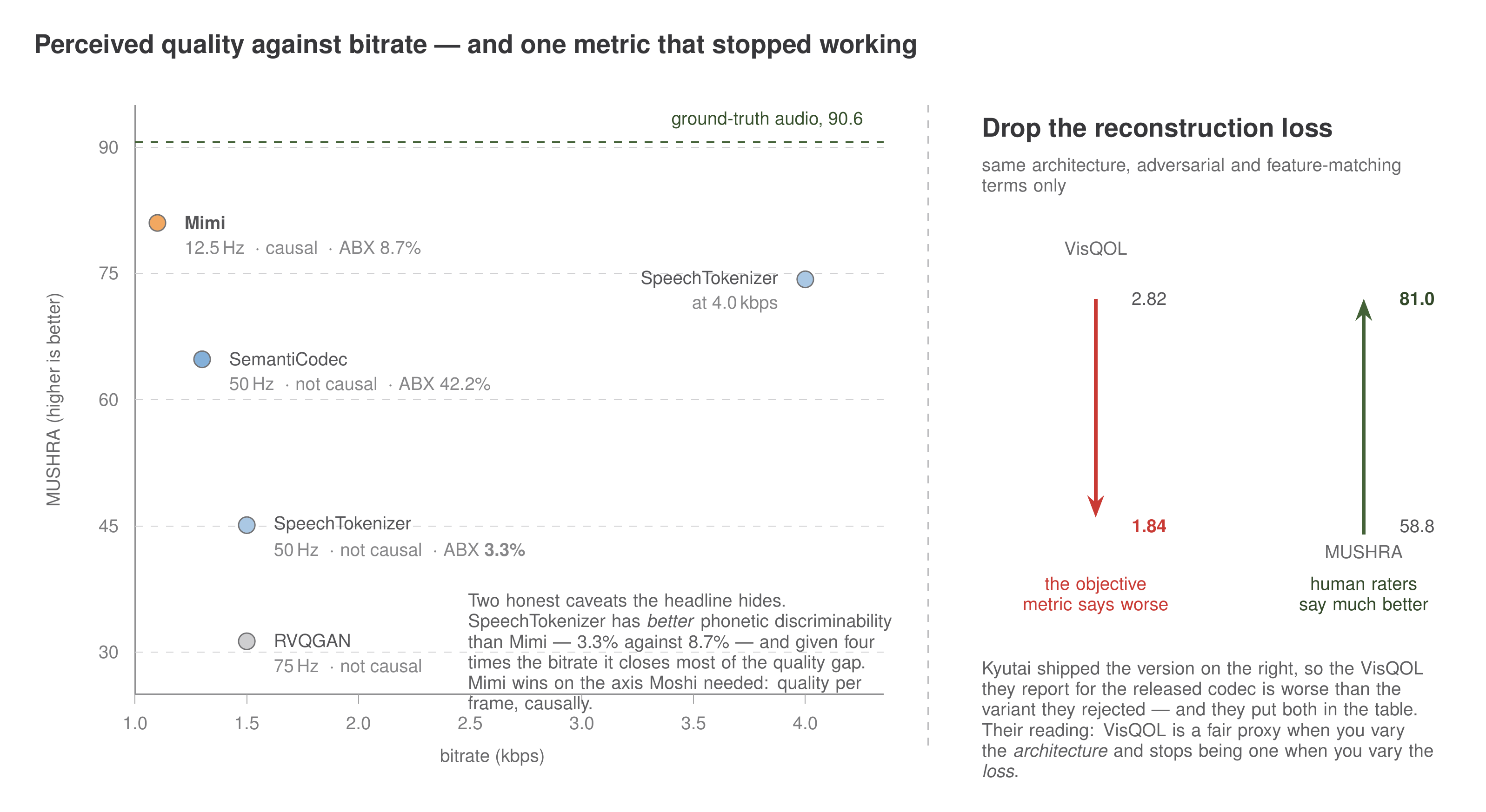
Figure 6 — Mimi wins on quality per frame; the instrument for measuring that stopped working.
Ravi: So it’s better on every axis at once.
Ana: On those axes. But their own conclusion is the more important output: when you change the training objective rather than the architecture, VisQOL and MOSNet move in directions uncorrelated with human perception. They note VisQOL is a reasonable proxy when you’re varying the generator architecture, and stops being one when you vary the loss.
Ravi: That’s not a small problem for the field.
Ana: It’s a blocking problem, and it’s the “what next” I care most about. Every automated pipeline downstream of audio quality inherits it. You can’t do reward-model training on perceived speech quality if the reward doesn’t track perception. You can’t do large-scale architecture search. You can’t even do honest leaderboards. Right now the field’s instrument for its primary output quantity is a twenty-person MUSHRA study, and that doesn’t scale to anything.
The RQ-Transformer: delay or depth, pick one
Ravi: Now the generative model. Seventeen tokens per timestep — how do you predict seventeen correlated integers at once?
Ana: Three options were on the table. Flatten them into seventeen sequence positions: that multiplies sequence length by seventeen and asks for 212 forward passes a second. Dead.
Ravi: Second?
Ana: Predict each codebook with its own independent classification head, and repair the independence assumption with a delay pattern, which is what MusicGen does. Codebook k is emitted k steps after codebook 1, so by the time codebook 3 is predicted, codebooks 1 and 2 for that frame are already in the past and visible to the temporal model. Elegant. But eight codebooks means eight steps of delay, and at 12.5 Hz that’s 640 milliseconds.
Ravi: Fine for music. Fatal here.
Ana: Fatal for a model whose entire premise is answering inside 200. So option three: the RQ-Transformer, borrowed from autoregressive image generation. Two transformers, nested. A large Temporal Transformer — 32 layers, dimension 4096, MLP dimension 11264, 32 heads, initialised from Helium — runs once per timestep over a 3,000-frame context, about four minutes, and emits a single context vector for that frame. Then a small Depth Transformer — 6 layers, dimension 1024, 16 heads — runs inside the frame, stepping through the seventeen sub-sequences one at a time, conditioned on that context vector and on the sub-sequences already decoded at the same timestep.
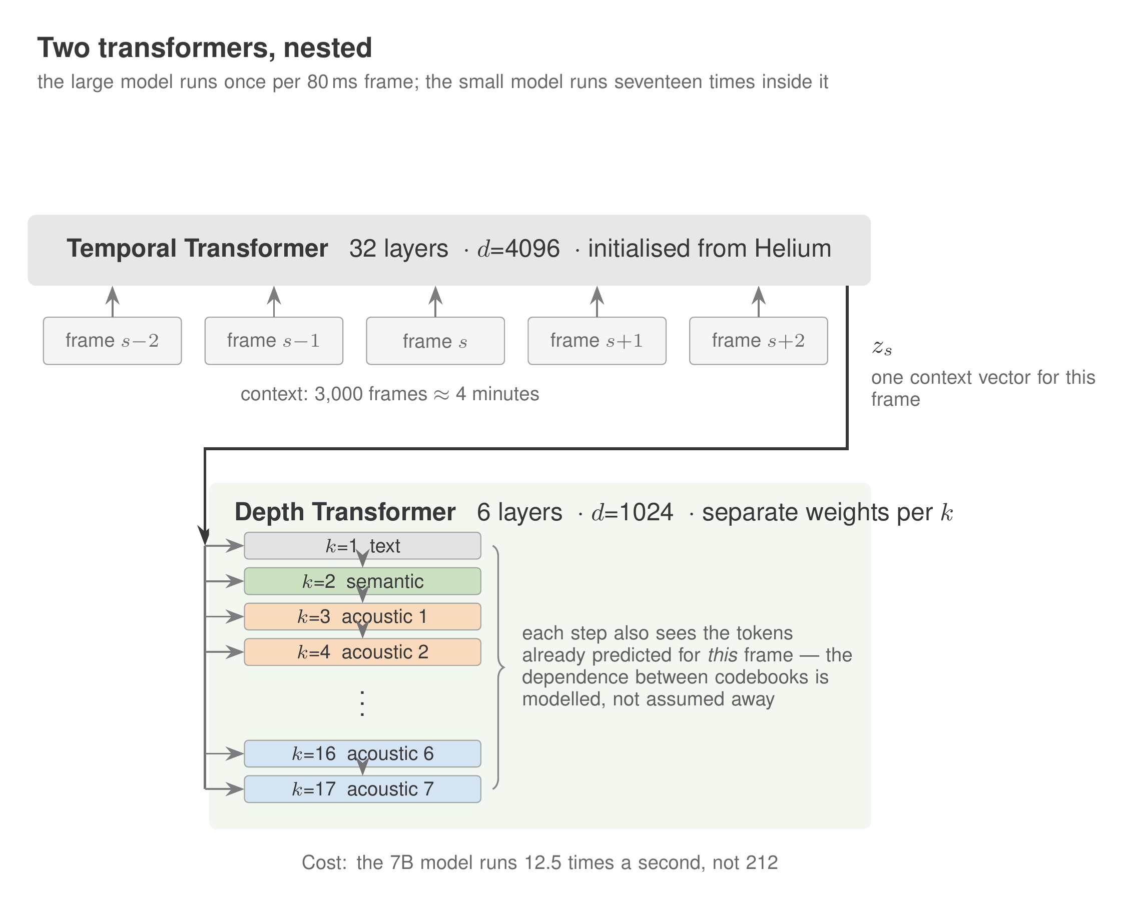
Figure 7 — A large model along time, a small model along depth.
Ravi: So you model the codebook dependencies explicitly instead of decorrelating them with delay.
Ana: And here’s the ablation, which says something sharper than “our thing is
better”. At the MusicGen-style delay pattern [0,1,2,3,4,5,6,7], adding the
RQ-Transformer barely helps — perplexity 42.2 to 40.3. You’d look at that and
conclude the complexity isn’t worth it.
Ravi: And at low latency?
Ana: At [0,2,2,2,2,2,2,2] — 240 milliseconds instead of 640 — the same
comparison is 135.4 to 36.8.
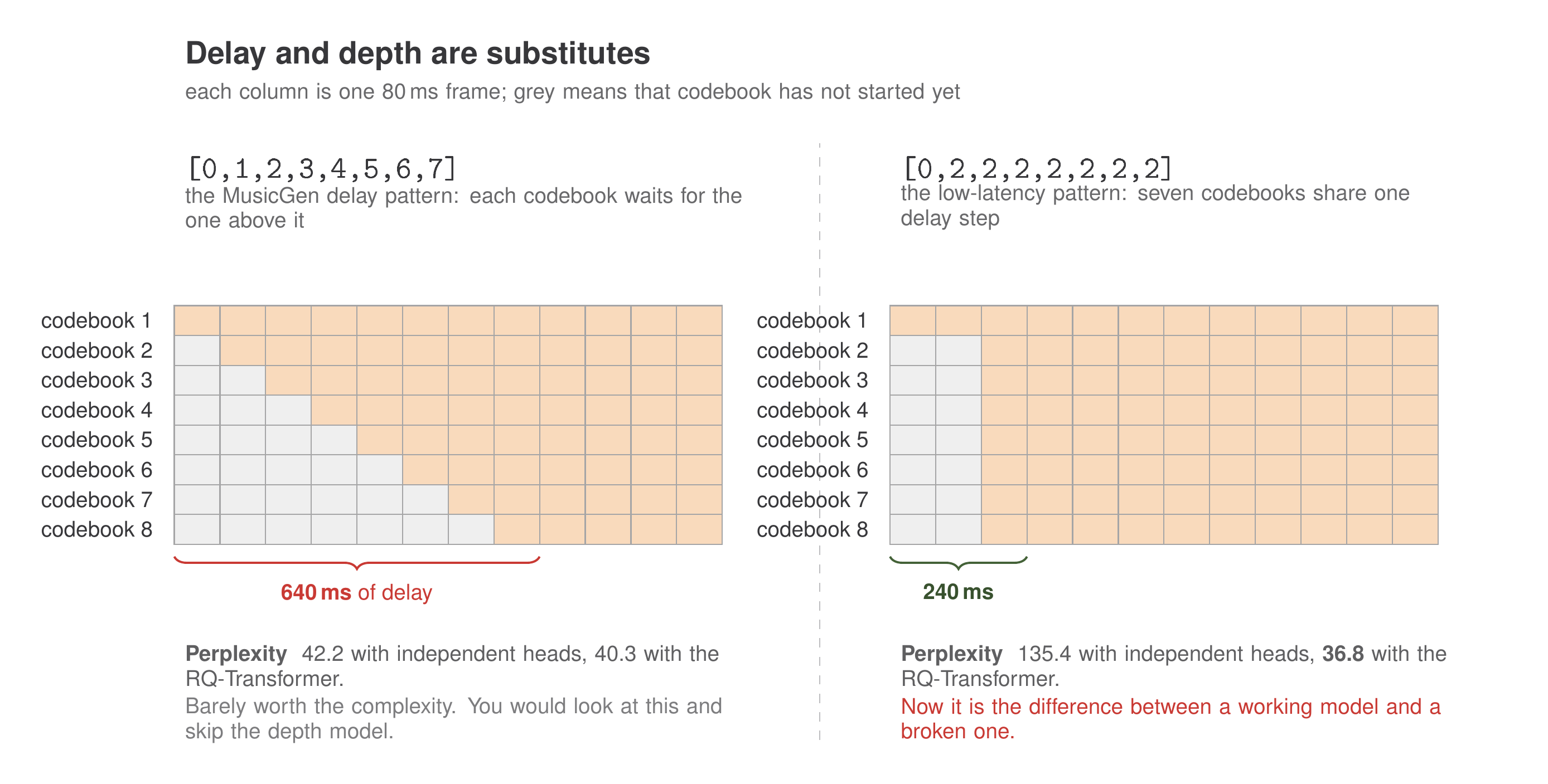
Figure 8 — The RQ-Transformer is not a general improvement; it is what you need once delay is spent.
Ravi: Oh, that’s a completely different claim.
Ana: It’s the claim I’d put on the poster. The RQ-Transformer is not a general-purpose improvement to audio language models. Delay and depth are substitutes. You can buy conditional independence between codebooks with latency, or you can model the dependence directly with a depth model. Moshi can’t afford the latency, so it pays with depth. If you have 640 milliseconds to spare, you don’t need any of this.
Ravi: Why isn’t the delay zero, then?
Ana: Because zero is measurably worse. Going from delay 0 to delay 1 improves generated speech quality enough to be worth the 80 milliseconds, and 2 helps a little more. They pre-train with delay 2 and fine-tune with delay 1, so the shipped model is 80 ms of frame plus 80 ms of delay: 160 total.
Ravi: Two more details I saw in the tables. Depthwise parametrisation and a semantic loss weight of 100.
Ana: Both are about the same underlying problem, which is that the seventeen sub-sequences compete. Depthwise parametrisation means separate weights per index k in the Depth Transformer, rather than shared weights across all seventeen — predicting a text token, a semantic token, and acoustic residual six are different jobs. Because the Depth Transformer is small, per-index parameters cost nothing at inference. And the loss weight: they set the semantic token’s cross-entropy weight to 100 while every other audio token stays at 1, because the levels were fighting and level one matters most for intelligibility.
Ravi: Blunt.
Ana: Extremely blunt, and it works — it’s a visible jump in the ablation table. The “what next” here is that depth models are now standard equipment, and the interesting question is whether the depth dimension has to be sequential at all. Seventeen sequential steps inside every frame is a hard serialisation. There’s real work on predicting the whole codebook stack in one shot with a masked or diffusion head, and if that lands, the depth transformer becomes a transitional artefact.
Multi-stream: the component that isn’t there
Ravi: Now the part I actually came for. How does it model me?
Ana: Take the user’s audio, encode it with the same Mimi, and concatenate its eight codebooks onto the sequence. That’s it. Seventeen sub-sequences per frame: one text, eight for Moshi, eight for the user. K equals 2Q plus 1.
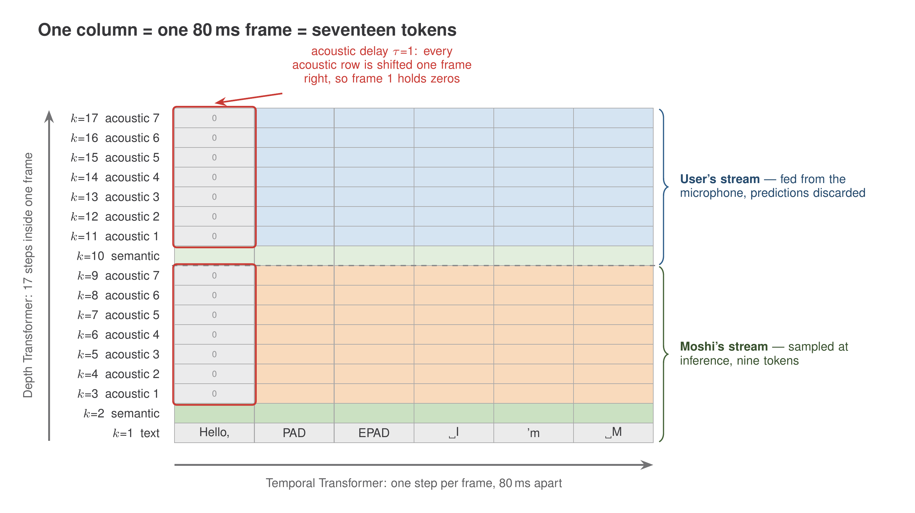
Figure 9 — One frame, seventeen tokens, every 80 milliseconds.
Ravi: That’s genuinely all of it?
Ana: That’s genuinely all of it, and the absence is the design. No cross-attention towers, which is what dGSLM used — a dual-tower architecture with cross-attention between the two channels. No interruption token, which is what LSLM used. No speaker-turn embeddings. Nothing that names a turn anywhere in the architecture.
Ravi: What happens at inference to the eight user columns?
Ana: Nine of the seventeen are sampled — Moshi’s text and Moshi’s audio — and the other eight are fed in from the microphone. The model’s own predictions for the user are computed and discarded.
Ravi: Then why train them at all? That’s wasted capacity.
Ana: Because it’s not wasted, it’s a free simulator. Since the model can predict both sides, you can generate entire two-party conversations with no human in the loop, and then measure the conversational dynamics offline. That is how the paper produces turn-taking statistics at all.
Ravi: What do those look like?
Ana: They follow the dGSLM methodology — inter-pausal units, pauses, gaps, overlaps. At temperature 1.0 Moshi produces IPU 50.8 seconds, pause 7.0, gap 4.5, overlap 4.1, against ground truth 51.1, 6.4, 4.2, 3.3. And on linguistic quality, scored by an external dialogue model, Moshi comes in at 41.9 perplexity against 45.9 for a cascaded topline and 195.9 for dGSLM.
Ravi: So the previous full-duplex model was fluent and empty.
Ana: dGSLM had conversational dynamics without conversational content. It produced startlingly natural laughter, overlap and well-timed backchannels from two-channel Fisher audio with no text anywhere — and it ran offline, modelled only semantic tokens, and had no text language model behind it. So the state of the art in early 2024 was a fork: a system that knew things and talked like a walkie- talkie, or a system that talked like a person and knew nothing. Moshi is the paper that refused the fork.
Ravi: Where has multi-stream gone since?
Ana: It turned out to be the most portable piece. Kyutai reused the same architecture for Hibiki, their simultaneous speech translation model — source speech in one stream, target speech in another, at the same 12.5 Hz, which lets it translate continuously instead of waiting for the utterance to end. That’s a completely different task with the same primitive.
Ravi: And the limitation?
Ana: Two streams is hard-coded into the shape. Three-party conversation, meetings, a model that has to attend to a room — none of that is a config change. And the deeper asymmetry is the one we’ll hit in the next section: Moshi’s own stream gets a text scaffold, and yours doesn’t.
Inner Monologue: text without a text pipeline
Ravi: This is the part that confused me most. It’s a speech-to-speech model that generates text. Isn’t that the thing we were trying to get away from?
Ana: The distinction is when. SpeechGPT and Spectron use what the paper calls chain-of-modality: generate the complete text answer, then convert it to speech. That’s a cascade wearing a trenchcoat — you can’t emit the first phoneme until the last word is decided, so you’ve reintroduced both the latency and the turn structure.
Ravi: And Inner Monologue?
Ana: Interleaves. At every 80 ms frame the model predicts one text token, as the first sub-sequence of that frame, before the semantic token and before the acoustic tokens. Within a single timestep the hierarchy runs text, then semantic, then acoustic. Nothing waits for anything.
Ravi: But text runs at three or four tokens a second and frames run at 12.5. How do you align them?
Ana: Whisper’s word-level timestamps. A word starting at time t has its
tokens placed at frame ⌊12.5·t⌋, everything else is filled with PAD, and an
EPAD token is inserted in the frame just before each word begins.
W = [PAD] * n_frames                       # default state is "not speaking"
for word, start_s in whisper_word_timestamps:
    t = int(start_s * 12.5)                # snap the word onto the audio clock
    W[t - 1] = EPAD                        # "I am about to start" <-- the good idea
    for j, tok in enumerate(tokenize(word)):
        W[t + j] = tok
# Result: Hello, PAD EPAD ⎵I ' m ⎵M oshi PAD PAD PAD PAD ...
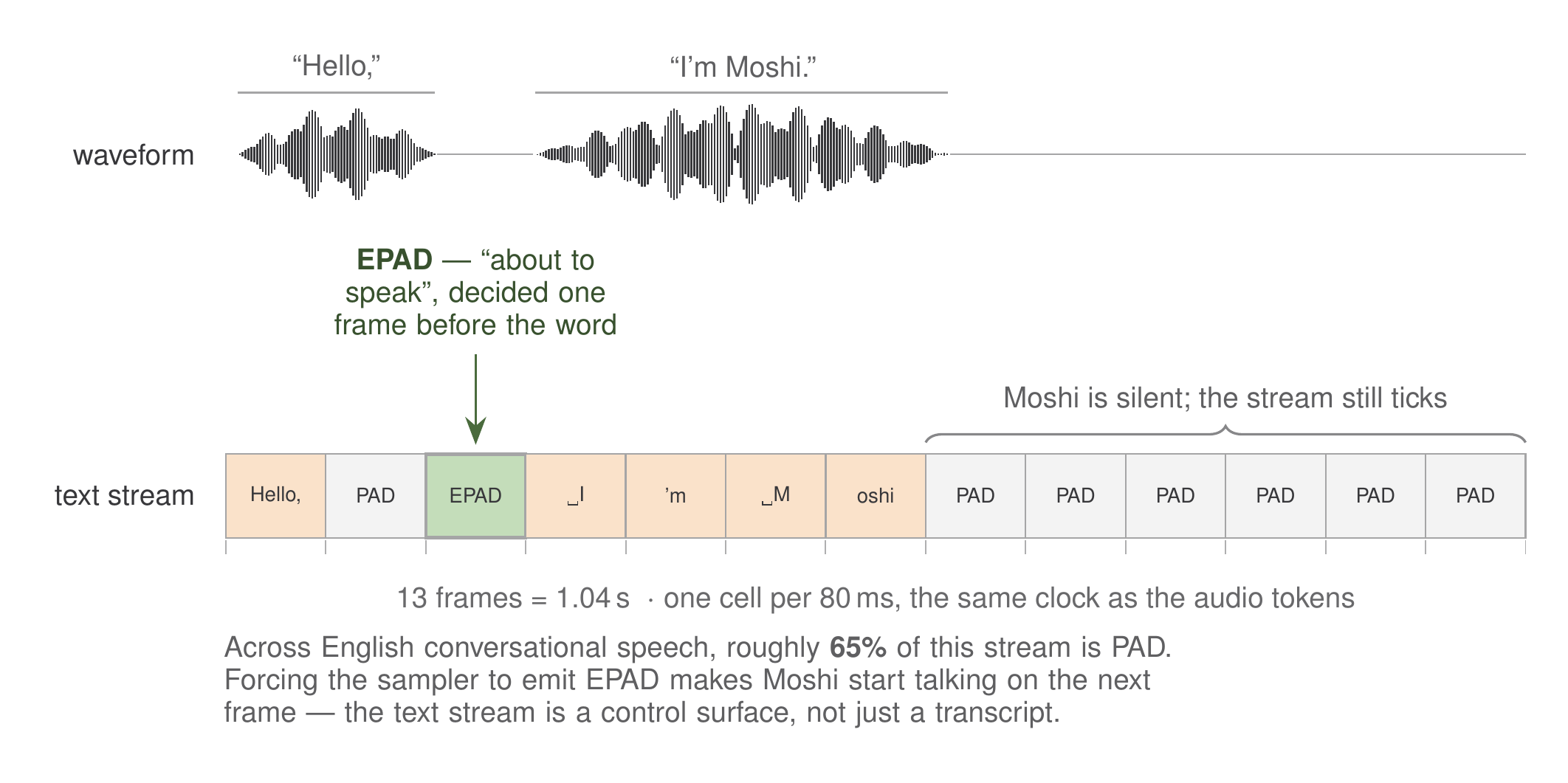
Figure 10 — Whisper’s word timestamps, snapped onto the audio clock.
Ravi: Why does EPAD need to exist? PAD already means “not speaking”.
Ana: Because without it, the model has to decide “stop padding” and “which word comes next” in a single prediction. EPAD splits that into two steps: first commit to speaking, then choose what to say. The paper describes it as useful guidance rather than strictly necessary — but it’s also precisely the hook that turns the text stream into a control surface. Force the sampler to emit EPAD and Moshi starts talking on the next frame.
Ravi: That’s a real product affordance. I can make it respond now without touching the audio path.
Ana: And in English conversational speech, about 65% of that stream is padding.
Ravi: What’s it worth?
Ana: It’s the single largest jump in every ablation the paper runs. Transcribed-generation NLL under an external scorer improves from 3.65 to 2.77, and the length of coherent generated speech goes from 602 characters to 1,920 — weak audio models collapse into silence, and this one stops collapsing. On spoken question answering it’s close to a tripling:
| Web Questions | LlaMA Questions | Audio Trivia QA | |
|---|---|---|---|
| Moshi, audio only | 9.2 | 21.0 | 7.3 |
| Moshi, Inner Monologue | 26.6 | 62.3 | 22.8 |
| SpeechGPT (7B) | 6.5 | 21.6 | 14.8 |
| Spectron (1B) | 6.1 | 22.9 | — |
| Helium (text, top line) | 32.3 | 75.0 | 56.4 |
The cost of that is one extra token per timestep. Seventeen instead of sixteen.
Ravi: And the delay thing? Someone told me you get ASR and TTS for free.
Ana: Almost literally free. The text stream and the audio streams are aligned with a delay, and the sign of that delay decides which modality leads. Put the text two seconds behind the audio, teacher-force the audio, sample only the text: the model transcribes what it hears. Streaming ASR, 5.7% WER on LibriSpeech test-clean, with word alignments accurate to 80 milliseconds.
Ravi: And the other direction.
Ana: Text two seconds ahead, teacher-force the text, sample the audio: the model speaks what it reads. Streaming TTS, 4.7% WER, against 5.9% for VALL-E — though VALL-E and NaturalSpeech 3 at 1.81% both see the entire utterance, while Moshi has two seconds of lookahead. Same loss, same architecture, same training data. One hyperparameter.
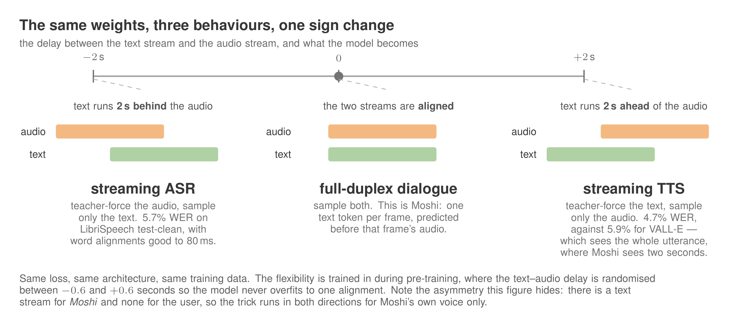
Figure 11 — One hyperparameter, three systems.
Ravi: Where did this idea end up?
Ana: Near-universal. Parallel text-and-speech generation is now the default in the omni-model line — you’ll find the same interleaved text channel, under various names, in most of the systems that shipped after. It’s arguably the most copied idea in the paper.
Ravi: And what’s left open?
Ana: Two things, and I think they’re the most interesting open problems in the paper. First: there is no text stream for the user. Moshi transcribes only itself. That was deliberate — real-time transcription of the user would mean an ASR component, internal or external, and that’s the thing the architecture exists to remove. But it means Moshi’s understanding of you is mediated entirely by audio tokens, while its own output gets text scaffolding. That asymmetry is almost certainly part of the knowledge gap we’re about to discuss.
Ravi: And the second?
Ana: Sixty-five percent of the text stream is PAD. That is an enormous
channel doing nothing, running at 12.5 Hz, already wired into the model’s residual
stream, at a moment when the model is listening rather than talking. If you
wanted a place to put deliberation — planning a response while the user is still
speaking, the way people actually do — it’s sitting right there, pre-built. There’s
early work pointing at exactly this.
The training ladder
Ravi: Let’s do training, because I suspect that’s where the actual difficulty was.
Ana: It’s four stages, and the shape of them tells you more about the field’s constraints than the architecture does.
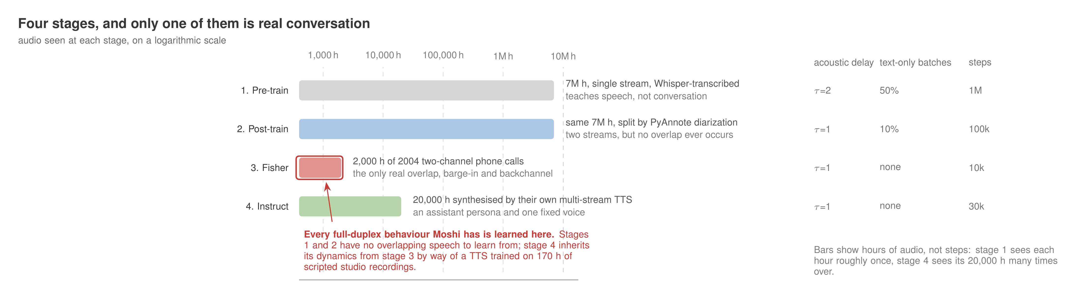
Figure 12 — Four training stages, and only one of them is real conversation.
Ana: Stage one, pre-training. Seven million hours of general audio, transcribed with Whisper large-v3, resampled to 24 kHz mono. Single stream — all speakers mixed together, and the text stream carries the words of everyone. One million steps, batches covering sixteen hours of audio, each item a five-minute sequence. They mask the text tokens 30% of the time and randomise the text-audio delay between minus and plus 0.6 seconds. Half the batches are text-only.
Ravi: Randomising the delay during pre-training — why?
Ana: So the model doesn’t overfit to one alignment, which is what later lets a single delay hyperparameter switch it between ASR, dialogue and TTS. The flexibility is trained in at this stage.
Ravi: Stage two.
Ana: Post-training, where it gains multi-stream. They diarise the same seven million hours with PyAnnote, sample one speaker as “main”, and use the diarization mask to split the waveform into two: the chosen speaker, and the residual. Those become the two input streams. Text stream carries only the main speaker. Delay fixed at zero. 100,000 steps, eight-hour batches, 10% text-only batches.
Ravi: Hang on. A diarization mask produces a hard partition.
Ana: Which means no overlap ever occurs, and the inactive stream is perfectly silent. The paper says this outright. It’s a good pre-training task for the two-stream format, and it teaches nothing about full-duplex dynamics.
Ravi: So where do the dynamics come from?
Ana: Stage three. Fisher. Two thousand hours of 2004-era telephone conversations between randomly paired strangers given a topic to discuss, recorded with each side on a separate channel, upsampled from 8 kHz to 24 kHz with AudioSR. Ten thousand steps, forty-minute batches, no more text batches. To get reliable timestamps despite long silences in each channel, they use whisper-timestamped with the medium model rather than the large one.
Ravi: Two thousand hours.
Ana: Two thousand hours. Every genuine overlap, barge-in and backchannel in the shipped model traces to that corpus.
Ravi: That’s the number I’d have led the paper with, honestly. Everything else scales — you can always get more unlabelled audio. That doesn’t.
Ana: It’s the field’s actual bottleneck and it’s structural: you need both sides of a conversation on separate channels, which basically means telephony archives or purpose-built recording. Stage four is where they work around it.
Ravi: Instruct tuning.
Ana: Twenty thousand hours of synthetic speech. They fine-tune Helium on Open Hermes and real conversation transcripts, use it to write dialogue between a user and an assistant, then speak those transcripts through a multi-stream streaming TTS built from the same architecture. 30,000 steps, 2.7-hour batches.
Ravi: Why not use a text instruct dataset directly?
Ana: They tried. Open Hermes and its relatives are formatted for reading, not speaking — URLs that can’t be rendered, bullet points, long enumerations. Question and answer shapes that no one uses out loud. So they generated oral-flow data instead, prompting for short turns and explicitly for backchanneling.
Ravi: What’s in that synthetic set?
Ana: More variety than I expected. General-knowledge conversations seeded from Wikipedia paragraphs and StackExchange posts, so the topic coverage is broad. Conversations about Moshi and Kyutai themselves, so it can answer “what are you”. Voice-instruction interactions — speak like a pirate, speak angrily — built by sampling a voice adjective and a character independently, so the combinations are deliberately unrelated. Roleplay scenarios. Deliberately misspelled user questions, followed by Moshi asking for clarification. Questions containing false premises — is the Eiffel Tower in Beijing — so it learns to say no, because otherwise almost every training conversation has it agreeing. Basic arithmetic and trivia, because they noticed it was bad at adding numbers. And safety conversations where the user asks for something unethical and Moshi refuses.
Ravi: That last set of choices is a product decision, not a research one.
Ana: Most of stage four is. And so is the augmentation, which is the part I’d call the difference between a demo and a thing that survives a real room. On the user’s stream: random gain between minus 24 and plus 15 dB half the time. Noise from the Deep Noise Suppression challenge 30% of the time, concatenated to cover the full duration, with the level sampled relative to the source — and crucially, half the time they splice in up to 30 seconds of silence, so the model experiences conditions changing from noisy to quiet and back.
Ravi: And echo?
Ana: This is the good one. They add a scaled-down copy of Moshi’s own output into the user’s stream, scaled by a factor sampled from 0 to 0.2, delayed between 100 and 500 milliseconds. Plus a reverb augmentation, applied together with the echo 30% of the time.
Ravi: Because otherwise it hears itself through the speaker and interrupts itself.
Ana: Every full-duplex system has this problem the moment it leaves headphones, and most of them solve it with acoustic echo cancellation in the audio stack. Kyutai trained it in.
Ravi: Scale?
Ana: 127 DGX nodes, 1,016 H100s, on Scaleway. FSDP and activation checkpointing throughout. AdamW with weight decay 0.1, and the learning rates step down by roughly an order of magnitude per stage — 3e-5 for the Temporal Transformer at pre-training, down to 2e-6 at instruct.
Ravi: So what’s the “what next” for training?
Ana: Synthetic full-duplex data, and it’s already where the field went. Everyone hit the Fisher wall and everyone’s answer is to generate two-channel conversations with LLMs plus a voice-cloning TTS. Which works, and imports a subtle problem: your synthesised dynamics are only as good as the model that generated them, and that model learned its dynamics from Fisher. There’s a lineage back to 2,000 hours of phone calls underneath a lot of what looks like scale.
Running it: quantization and what it costs
Ravi: Deployment. What does it actually take?
Ana: In bfloat16 the released models are about 7.7 billion parameters and want roughly 16 GB. Practical end-to-end latency is around 200 milliseconds on an L4 — so 160 theoretical, 200 real, and the 40 milliseconds of slack is the inference stack.
Ravi: And quantized?
Ana: They studied post-training quantization properly, which is rare for a speech paper. Activations in bfloat16, dynamically quantized to 8 bits with symmetric AbsMax at the input of every linear layer. Weights asymmetric MinMax at various bitwidths and block sizes. Both transformers quantized. Left alone: the initial embedding layers for text and audio, the RMSNorms, and Mimi itself.
Ravi: Findings?
Ana: Three that matter to you. First, the Depth Transformer is robust — keeping it in high precision doesn’t meaningfully improve audio quality, so don’t spend your precision budget there. Second, block size matters more than you’d guess: at 4-bit weights, Helium holds within about two MMLU points of the floating-point baseline with blocks of 32, but drops to 49.29 per-channel. Third, and the one I’d flag: Helium is more robust to quantization than Moshi is. The audio model degrades faster than the text model it came from.
Ravi: Which suggests the audio path is using its precision.
Ana: That’s my read. And they note audio degradations that the linguistic metrics don’t capture at all — you can hold MMLU roughly flat and still make the voice worse. Which is the metrics problem again, arriving from a different direction.
Safety: one thing that worked, one that didn’t
Ravi: Voice consistency. How do you stop an open-weights speech model impersonating people?
Ana: For its own voice, they got a clean result: conditioning the instruct- tuning TTS on a single voice actor — who recorded monologues across more than seventy speaking styles — was sufficient. No inference-time control needed. The model essentially never uses another voice for itself. Meanwhile the user’s stream voice is randomised per example, which buys robustness to accents and recording conditions.
Ravi: That’s a nice result. Persona through data, not constraints.
Ana: And now the one that didn’t work. They tested AudioSeal, a state-of-the- art audio watermarking method, on Moshi’s output. Unwatermarked audio scores 0.0855 on the detector. Watermarked and unmodified: 0.9999. Add pink noise and it degrades but survives on long clips. Then compress and decompress.
Ravi: Through what?
Ana: Through RVQGAN, detection falls to 0.1101. Through Mimi itself, 0.0805 — on ten-second clips, below the score of audio that was never watermarked at all.
Ravi: Their own codec is the attack.
Ana: And it’s not a bug, it’s the definition. A low-bitrate codec discards everything not needed for reconstruction, and an imperceptible watermark is by construction not needed for reconstruction. They explored watermarking in the token space instead and report it as a negative result — the tokens aren’t stable through re-encoding. They list ideas for fixing it: mark only the first RVQ levels, add an idempotence loss so tokens survive auto-encoding, train for tolerance to temporal shift.
Ravi: And with open weights there’s a simpler problem.
Ana: They name it directly: for one well-known open image model, removing the watermark required commenting out a single line. Any watermark you can disable in the inference code is a watermark for honest users only.
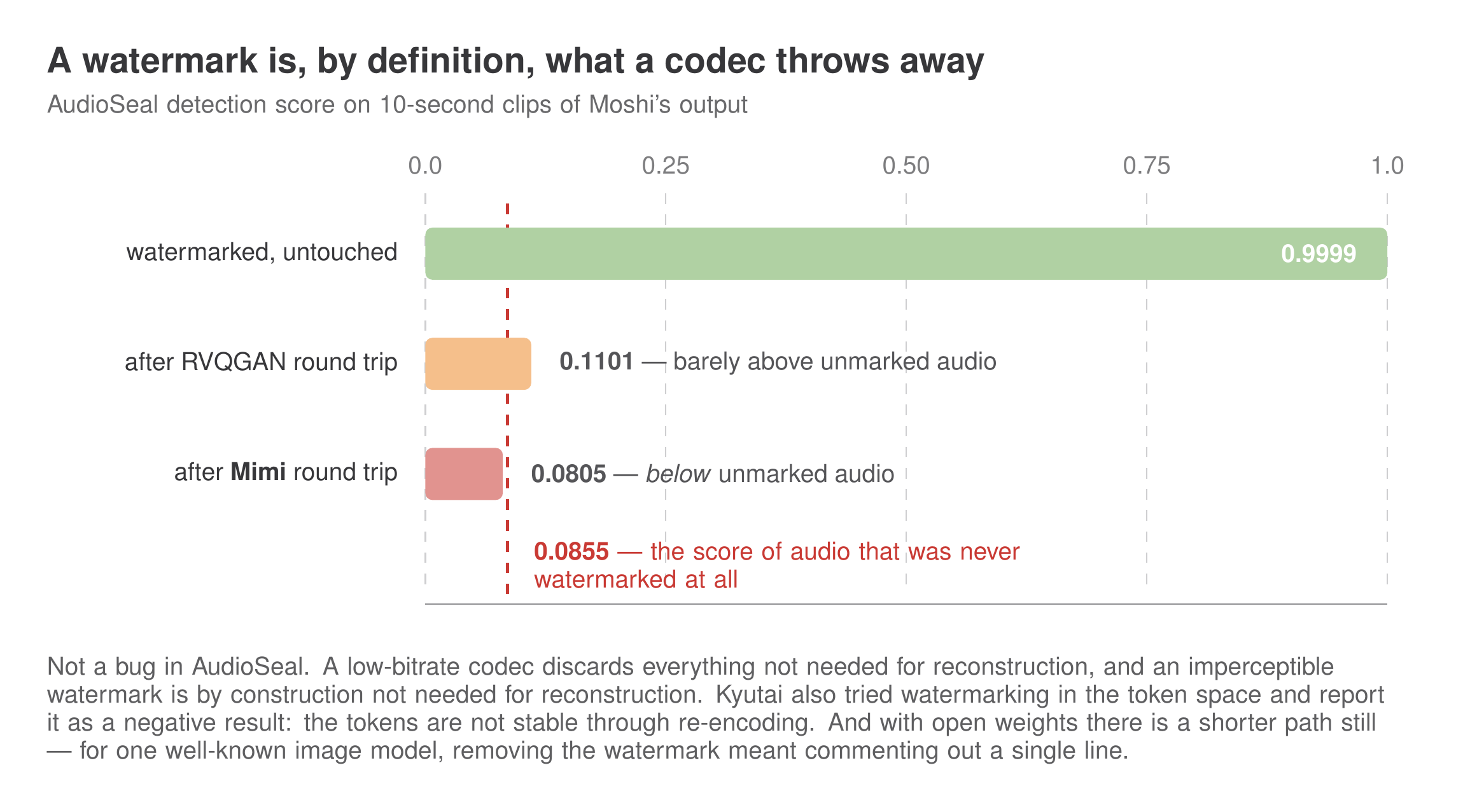
Figure 13 — The codec is the attack.
Ravi: So where does that leave provenance for speech?
Ana: Unsolved, and I’d say more unsolved than for images, because the compression ratios are brutal and re-encoding is routine rather than adversarial. Every phone call, every messaging app, every video platform re-encodes. The most promising direction in their discussion is watermarking through the training data rather than the output — the radioactive-data line of work — but that identifies a model, not a clip.
Evaluation: the instruments arrived after the models
Ravi: Last technical piece. How do we know any of this is good?
Ana: Partly we don’t, and the paper is unusually honest about which parts. Start with the knowledge tax. Helium scores 54.3 on MMLU; Moshi 49.7. On Trivia QA the gap is not subtle — 56.4 for text Helium against 22.8 for Moshi. Web Questions 32.3 to 26.6. LlaMA Questions 75.0 to 62.3.
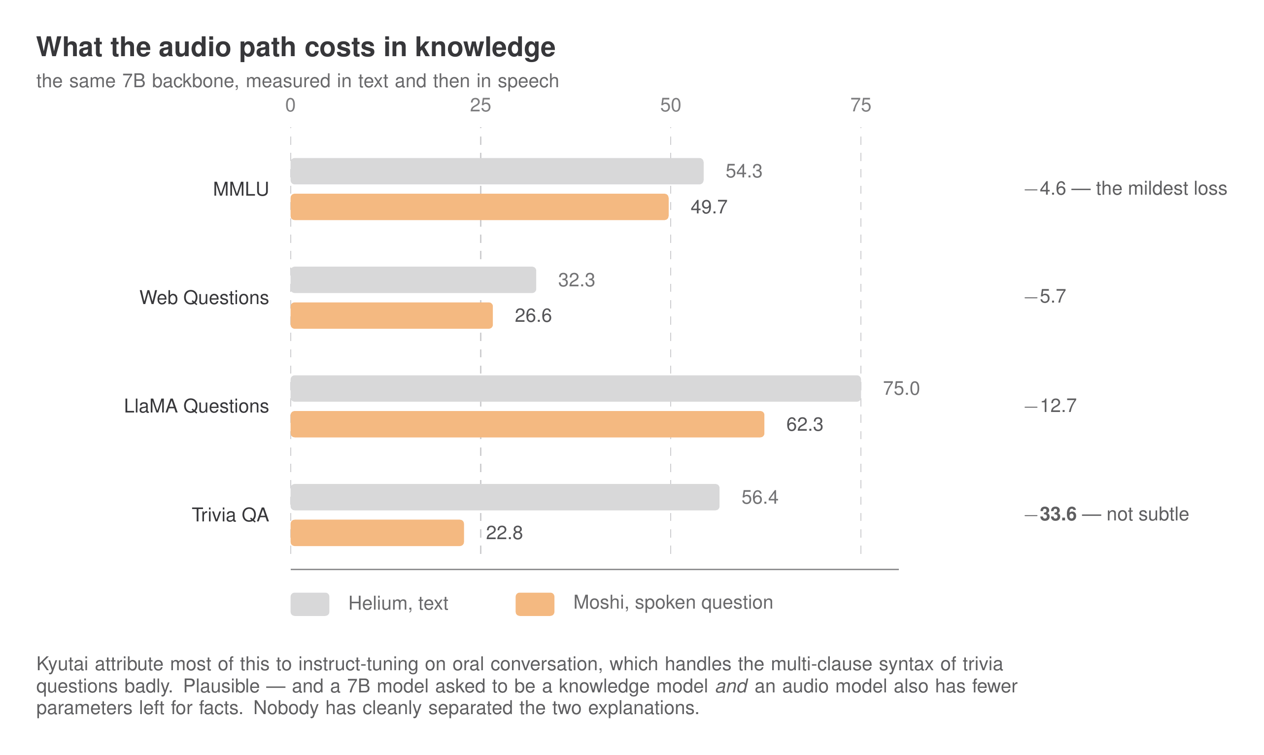
Figure 14 — The same 7B backbone, measured in text and then in speech.
Ravi: What’s their explanation?
Ana: Instruct-tuning on oral conversation. They inspect the errors and find multi-clause trivia questions and unusual syntactic structures are where it breaks — the example they give is a two-sentence question with the answer buried in a relative clause, which is a shape that never appears in spoken dialogue. Plausible, and I believe it explains part of the gap. But a 7B model asked to be both a knowledge model and an audio model has fewer parameters for facts, and I’d read some of that gap as a tax rather than an artefact.
Ravi: Is it recoverable?
Ana: That’s the open question the whole architecture rides on. If it’s fine-tuning distribution, more diverse instruct data fixes it. If it’s capacity, you need scale or a different graft. Nobody has cleanly separated those.
Ravi: And the speech metrics?
Ana: Weirder. After the fine-tuning that turns Moshi into a dialogue system, sWUGGY — a lexical-knowledge probe from the textless NLP suite — falls from 72.6 to 63.0. The authors argue the metric is misleading here and note they see no drop in lexical variety or intelligibility.
Ravi: Do you buy that?
Ana: Mostly. Those benchmarks were built for models trained on clean read speech, and Moshi trains on wildly varied acoustic conditions, which the paper argues decorrelates the metrics. But “our numbers went down and the metric is wrong” is a claim that needs an alternative measurement, and the alternative they offer is spoken question answering, which measures something different.
Ravi: What about the thing I actually care about — does it take turns well?
Ana: Here’s the gap. The turn-taking evaluation reports corpus-level aggregates against Fisher: IPU duration, pause, gap, overlap. Moshi matches ground truth closely at temperature 1.0. That tells you the distribution of behaviours is right.
Ravi: It doesn’t tell me whether it backchannels at the right moment.
Ana: It doesn’t. A model could produce a perfectly human-looking overlap histogram while overlapping in all the wrong places. Distributional match and moment-level correctness are different claims, and the paper can only make the first one, because in September 2024 there was nothing to make the second one with.
Ravi: And now?
Ana: Now there is. Full-Duplex-Bench arrived in March 2025 and evaluates specific behaviours: pause handling — does the model take over during a natural mid-sentence pause, measured as takeover rate; backchanneling, measured by frequency and by divergence from human timing; smooth turn-taking, measured by response latency; and interruption handling. A line of follow-on benchmarks extends it to overlap-heavy scenarios and multi-turn interaction.
Ravi: So the models shipped before the instruments.
Ana: Which is normal in a young area and worth saying out loud anyway, because it means every architectural claim in the 2024 papers — including Moshi’s — was validated against metrics that couldn’t see the behaviour the architecture was for. The models were built to handle overlap and evaluated on aggregate silence statistics.
Ravi: That’s the part I’d want a researcher to keep pulling on.
Ana: It’s where I’d put effort, yes. And there’s a layer past behaviour, which is whether the model does what it was told to do about turn-taking — hold the floor while I finish, don’t interrupt me in this context, be more or less interjective depending on who you’re talking to. Behavioural correctness averaged over a corpus and instructed behaviour on a given call are different targets, and the second one is barely measured at all.
What it changed, and what we do next
Ravi: Give me the verdict.
Ana: Moshi won the argument about latency and conversational dynamics decisively. The multi-stream primitive got reused for a different task by its own authors within five months. Inner Monologue — a time-aligned text channel interleaved with audio rather than preceding it — is now close to standard. Mimi’s combination of low frame rate, semantic distillation and causality became the default shape for a speech tokenizer, and the split RVQ is a small idea that generalises well past this paper.
Ravi: And the argument it lost?
Ana: Capability, at least for now, and the most honest evidence is that Kyutai shipped Unmute in 2025 — a cascaded stack. Their own streaming STT, an off-the- shelf text LLM, their own TTS. On their page for it they say plainly that while Moshi has unmatched latency and naturalness, it doesn’t yet match text models on function calling, stronger reasoning and in-context learning, and that Unmute exists to bring those to real-time voice. They also say they still believe the future is end-to-end.
Ravi: Both of those can be true.
Ana: Both are true, and holding them together is the correct summary of where the architecture stands. The capability frontier keeps moving in text, and a speech-native model has to re-earn each advance rather than inheriting it. That’s the structural disadvantage, and nothing in the Moshi paper solves it.
Ravi: So if you were picking problems.
Ana: Four, in the order I’d rank them. One: a perceptual quality metric that survives a change of training objective, because everything automated downstream is blocked on it. Two: full-duplex supervision that isn’t downstream of 2,000 hours of phone calls — which means either new recording at scale, or synthetic generation whose dynamics don’t inherit from Fisher through a TTS. Three: closing the knowledge gap without giving up the audio path, which probably means figuring out how to graft onto frontier text models rather than training your own Helium. Four: evaluation that measures the moment, not the distribution — and past that, whether the model follows instructions about how to take turns, which almost nothing currently measures.
Ravi: And the thing you’d build tomorrow?
Ana: Put something in the padding. Sixty-five percent of that text stream is
PAD, arriving at 12.5 Hz, while the model is listening rather than talking. It’s
the only place in any of these architectures where there’s obviously spare capacity
at exactly the moment a person would be thinking.
References
Moshi and what came out of it
-
Défossez, A., Mazaré, L., Orsini, M., Royer, A., Pérez, P., Jégou, H., Grave, E., & Zeghidour, N. (2024). Moshi: a speech-text foundation model for real-time dialogue. Kyutai technical report. arXiv:2410.00037. https://arxiv.org/abs/2410.00037 — code and weights at https://github.com/kyutai-labs/moshi; codec at https://huggingface.co/kyutai/mimi
-
Labiausse, T., Mazaré, L., Grave, E., Pérez, P., Défossez, A., & Zeghidour, N. (2025). High-Fidelity Simultaneous Speech-To-Speech Translation (Hibiki). ICML 2025, PMLR 267:32116–32129. arXiv:2502.03382. https://arxiv.org/abs/2502.03382 — the multi-stream architecture reused for simultaneous interpretation.
-
Kyutai (2025). Unmute. https://kyutai.org/unmute/ — the same lab’s cascaded stack, and their stated reasoning for building it.
Neural audio codecs
-
van den Oord, A., Vinyals, O., & Kavukcuoglu, K. (2017). Neural Discrete Representation Learning (VQ-VAE). NeurIPS. arXiv:1711.00937. https://arxiv.org/abs/1711.00937
-
Zeghidour, N., Luebs, A., Omran, A., Skoglund, J., & Tagliasacchi, M. (2021). SoundStream: An End-to-End Neural Audio Codec. IEEE/ACM TASLP, 30:495–507. arXiv:2107.03312. https://arxiv.org/abs/2107.03312 — origin of residual vector quantization for audio, and of quantizer dropout.
-
Défossez, A., Copet, J., Synnaeve, G., & Adi, Y. (2022/2023). High Fidelity Neural Audio Compression (EnCodec). TMLR. arXiv:2210.13438. https://arxiv.org/abs/2210.13438 — the reconstruction-plus-adversarial recipe Mimi departs from.
-
Kumar, R., Seetharaman, P., Luebs, A., Kumar, I., & Kumar, K. (2023). High-Fidelity Audio Compression with Improved RVQGAN. NeurIPS. arXiv:2306.06546. https://arxiv.org/abs/2306.06546 — source of the quantization-rate observation Mimi adapts.
-
Zhang, X., Zhang, D., Li, S., Zhou, Y., & Qiu, X. (2024). SpeechTokenizer: Unified Speech Tokenizer for Speech Language Models. ICLR 2024. arXiv:2308.16692. https://arxiv.org/abs/2308.16692 — the semantic-distillation idea the split RVQ extends.
Speech representations and audio language models
-
Chen, S., Wang, C., Chen, Z., Wu, Y., Liu, S., Chen, Z., et al. (19 authors) (2022). WavLM: Large-Scale Self-Supervised Pre-Training for Full Stack Speech Processing. IEEE JSTSP, 16(6):1505–1518. arXiv:2110.13900. https://arxiv.org/abs/2110.13900 — Mimi’s distillation teacher. Weights at https://huggingface.co/microsoft/wavlm-large
-
Lakhotia, K., Kharitonov, E., Hsu, W.-N., Adi, Y., Polyak, A., Bolte, B., Nguyen, T.-A., Copet, J., Baevski, A., Mohamed, A., & Dupoux, E. (2021). On Generative Spoken Language Modeling from Raw Audio (GSLM). TACL, 9:1336–1354. arXiv:2102.01192. https://arxiv.org/abs/2102.01192 — origin of the textless-NLP metric suite, including sWUGGY.
-
Borsos, Z., Marinier, R., Vincent, D., Kharitonov, E., Pietquin, O., Sharifi, M., Roblek, D., Teboul, O., Grangier, D., Tagliasacchi, M., & Zeghidour, N. (2023). AudioLM: A Language Modeling Approach to Audio Generation. IEEE/ACM TASLP, 31:2523–2533. arXiv:2209.03143. https://arxiv.org/abs/2209.03143 — the semantic-then-acoustic hierarchy Inner Monologue extends with a text prefix.
-
Nguyen, T. A., Kharitonov, E., Copet, J., Adi, Y., Hsu, W.-N., Elkahky, A., Tomasello, P., Algayres, R., Sagot, B., Mohamed, A., & Dupoux, E. (2023). Generative Spoken Dialogue Language Modeling (dGSLM). TACL, 11:250–266. arXiv:2203.16502. https://arxiv.org/abs/2203.16502 — the full-duplex predecessor, and Moshi’s dialogue-dynamics baseline.
Architecture and generation patterns
-
Lee, D., Kim, C., Kim, S., Cho, M., & Han, W.-S. (2022). Autoregressive Image Generation using Residual Quantization. CVPR 2022, pp. 11523–11532. arXiv:2203.01941. https://arxiv.org/abs/2203.01941 — where the RQ-Transformer comes from.
-
Copet, J., Kreuk, F., Gat, I., Remez, T., Kant, D., Synnaeve, G., Adi, Y., & Défossez, A. (2023). Simple and Controllable Music Generation (MusicGen). NeurIPS. arXiv:2306.05284. https://arxiv.org/abs/2306.05284 — origin of the codebook delay patterns Moshi measures against.
-
Radford, A., Kim, J. W., Xu, T., Brockman, G., McLeavey, C., & Sutskever, I. (2023). Robust Speech Recognition via Large-Scale Weak Supervision (Whisper). ICML. arXiv:2212.04356. https://arxiv.org/abs/2212.04356 — supplies both the pre-training transcripts and the word-level timestamps Inner Monologue is built on.
Conversation, data, and evaluation
-
Stivers, T., Enfield, N. J., Brown, P., Englert, C., Hayashi, M., Heinemann, T., Hoymann, G., Rossano, F., de Ruiter, J. P., Yoon, K.-E., & Levinson, S. C. (2009). Universals and cultural variation in turn-taking in conversation. PNAS, 106(26):10587–10592. https://doi.org/10.1073/pnas.0903616106 — the human turn-transition timings Moshi’s latency target is measured against.
-
Cieri, C., Miller, D., & Walker, K. (2004). The Fisher Corpus: a Resource for the Next Generations of Speech-to-Text. LREC 2004. https://aclanthology.org/L04-1500/ — the two-channel telephone corpus that supplies Moshi’s only real full-duplex supervision.
-
Lin, G.-T., et al. (2025). Full-Duplex-Bench: A Benchmark to Evaluate Full-duplex Spoken Dialogue Models on Turn-taking Capabilities. arXiv:2503.04721. https://arxiv.org/abs/2503.04721 — pause handling, backchanneling, smooth turn-taking, interruption. Code and later versions at https://github.com/DanielLin94144/Full-Duplex-Bench
-
San Roman, R., Fernandez, P., Elsahar, H., Défossez, A., Furon, T., & Tran, T. (2024). Proactive Detection of Voice Cloning with Localized Watermarking (AudioSeal). ICML 2024, PMLR 235:43180–43196. arXiv:2401.17264. https://arxiv.org/abs/2401.17264 — the watermarking method Mimi erases.
-
Can Speech LLMs Think while Listening? arXiv:2510.07497. https://arxiv.org/abs/2510.07497 — chain-of-thought inside a multi-stream speech LM; the direction Ana points at in the padding discussion. [Author list unverified — complete before publishing.]