Evolving Voices: How Speech Became a Language Modeling Problem

Open a text file and the vocabulary is already there. Words, or subwords, sitting in a finite list you can index into and take a softmax over. Nobody had to invent it; writing systems did that work centuries ago.

Now open an audio file. One second of 16 kHz speech is sixteen thousand floating-point numbers. There are no words in it. There are no boundaries between words in it. There is not even a fixed number of things per second — a phoneme might last 30 milliseconds or 300, and nothing in the signal marks where one ends. If you want to run a language model over speech, the first problem is not the model. It is that speech has no alphabet, and you have to build one.

This post walks through the architectures that built it, and how each one works internally. The story runs from 2020 to 2023 and splits neatly into two halves: a group of self-supervised encoders that learned to hear, and a group of generative models that used the resulting tokens to speak.

Terms you’ll need

Discrete tokens are slices of continuous audio mapped onto a finite alphabet. Every system here produces or consumes them. They are what makes a softmax possible.

Semantic tokens encode linguistic content — roughly, which phoneme was uttered. They are compact, stable over long spans, and audio reconstructed from them sounds bad.

Acoustic tokens encode the signal itself: timbre, room reverberation, breathiness, prosody. They reconstruct faithfully and lose coherence over long generated sequences.

Frame rate is how many tokens per second the encoder emits. Nearly everything below runs at 20 ms per frame (50 Hz), for reasons that trace back to one architectural choice in 2020.

Masked prediction is the training scheme shared by all three encoders: hide part of the input, ask the model to recover something about the hidden part from what remains.

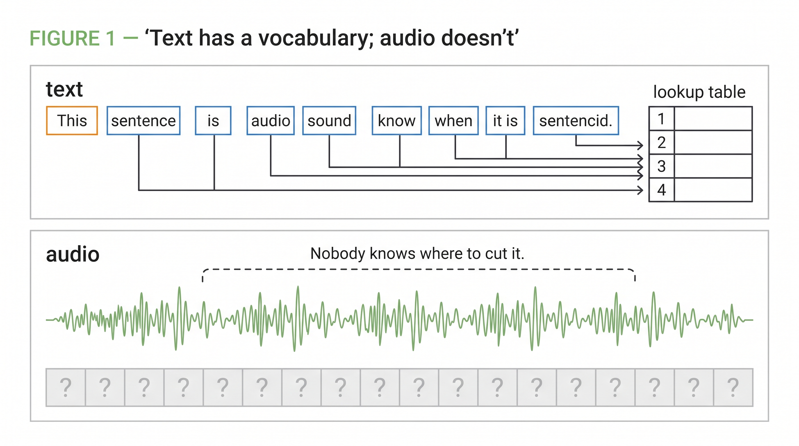
Figure 1 — Text arrives pre-segmented into a finite vocabulary; audio is a continuous stream with no boundaries given.

Why not just use an existing audio format?

This is the question to answer before anything else, because the alternative seems obvious. MP3 already compresses audio. Why invent a new representation?

Two reasons, and they are different from each other.

The first is that MP3 is compressed for ears. It is a continuous, perceptually-tuned representation — a set of real-valued coefficients, not a selection from a finite set. There is nothing to predict a distribution over. A language model’s entire mechanism is assigning probability mass across a fixed vocabulary, and a perceptual codec doesn’t have one.

The second is length. Even if you discretized MP3 coefficients somehow, you would still be handling thousands of units per second. Self-attention costs grow quadratically with sequence length, which caps practical contexts in the low thousands of tokens. A one-minute exchange has to fit in that budget alongside everything else the model needs to remember.

So the requirements are specific: a finite vocabulary, a frame rate low enough that a minute of audio is a manageable number of tokens, and enough information retained that you can still reconstruct something worth listening to. The systems below are different resolutions of those three constraints.

The core idea

Speech carries two kinds of information — what was said, and how it sounded — and the representation you get depends entirely on which one you optimized for. Encoders trained to support recognition learn to discard the speaker. Codecs trained to support reconstruction learn to keep everything and, in doing so, keep no linguistic structure. Understanding any architecture below means asking which of the two it was built for, and what it did about the other.

This is measurable, and it was measured directly. Comparing the two token families on the same speech data, semantic tokens from w2v-BERT scored 6.7 / 7.6 on within- and across-speaker phonetic discriminability (ABX error rate, lower is better) but only 1.1 on reconstruction quality (ViSQOL, higher is better). Acoustic tokens from SoundStream at 2000 bps came out at 22.4 / 28.7 on ABX and 3.3 on ViSQOL. Each alphabet is worst at exactly what the other is best at.

Hold onto those four numbers. They are the reason the second half of this post looks the way it does.

Part one: encoders that learn without labels

Three models, all trained on unlabeled audio, all using masked prediction, all differing in what they ask the model to predict about the masked region. That one difference is the whole design space.

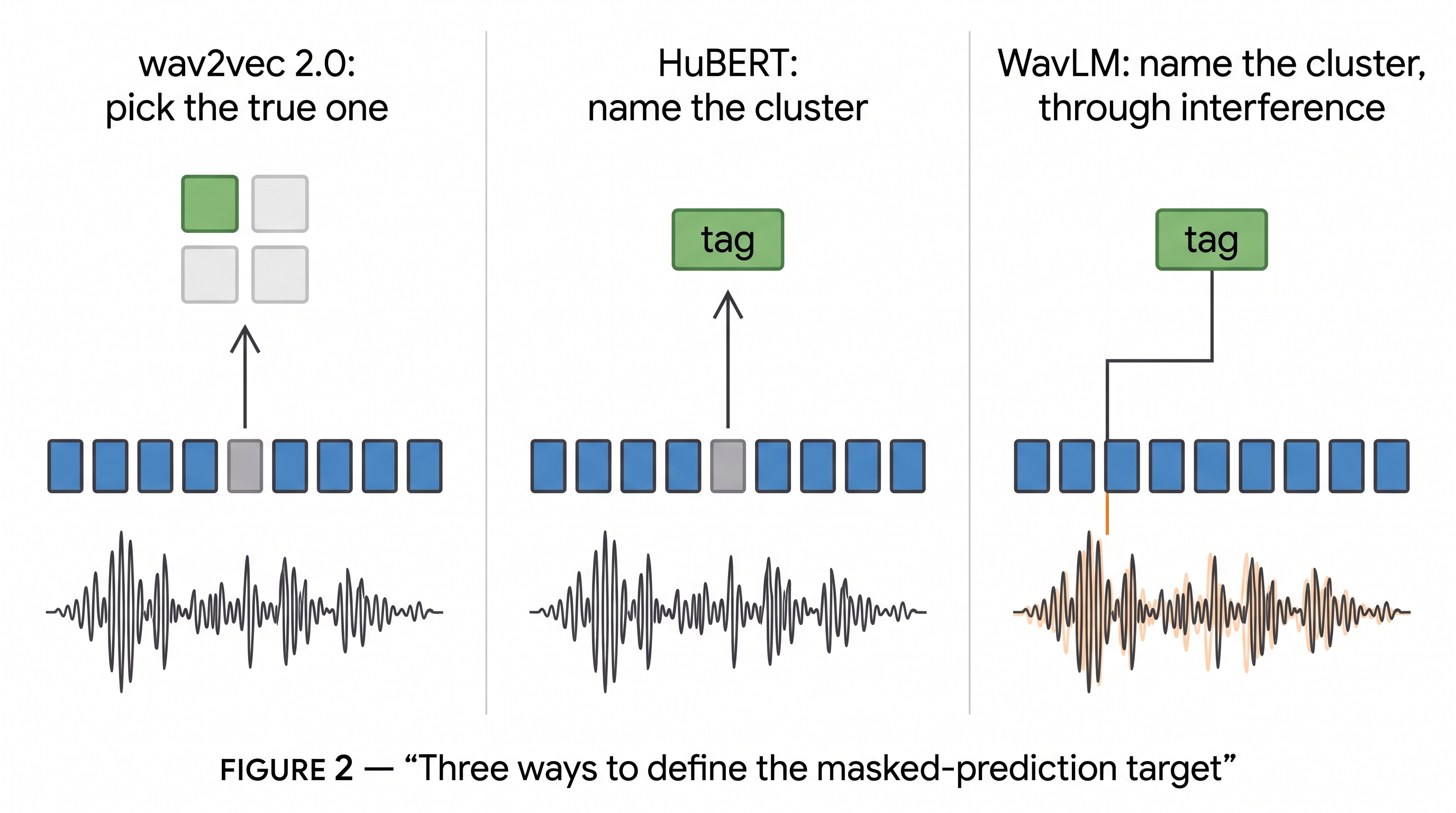
Figure 2 — The three self-supervised encoders differ only in what they ask the model to predict about the masked region.

wav2vec 2.0 (2020)

wav2vec 2.0 showed that representations learned from raw audio alone, then fine-tuned on a small amount of transcribed speech, could beat the best semi-supervised methods while being conceptually simpler.

Three components, and the relationship between them is the contribution.

The convolutional feature encoder takes the raw waveform and produces a sequence of latent frames. Seven blocks, 512 channels each, strides (5,2,2,2,2,2,2), kernel widths (10,3,3,3,3,2,2). Multiply the strides together and you get 320 — so 16,000 samples per second become 50 frames per second, one every 20 ms, each with a 25 ms receptive field. This is where the field’s standard frame rate comes from. HuBERT and WavLM adopt the identical encoder.

The Transformer context network builds contextualized representations across those frames. It does not use learned absolute position embeddings; a convolutional layer with kernel size 128 and 16 groups plays the role of a relative positional embedding, its output added to the input before layer norm.

The quantization module produces the discrete targets, and it’s worth slowing down here because the trick recurs everywhere in this field.

You want a large vocabulary of speech units. Storing a large codebook is expensive and, worse, most entries go unused. Product quantization gets around this by splitting the representation into groups and quantizing each group separately. With G codebooks of V entries each, you pick one entry from each and concatenate. wav2vec 2.0 uses G=2 and V=320, which yields a theoretical maximum of 320 × 320 = 102.4k distinct codewords from only 640 stored vectors.

Picking an entry is an argmax, which has no gradient. The fix is a Gumbel softmax with a straight-through estimator: the forward pass takes the hard argmax, the backward pass uses the gradient of the soft distribution. Temperature τ anneals from 2 down to 0.5 during training, so the selection starts soft and sharpens.

Training. Mask spans in the latent space, then identify the true quantized latent for each masked step among distractors:

# wav2vec 2.0 pre-training, one step.

z = conv_encoder(waveform)              # 50 Hz latent frames
q = quantize(z)                         # product-quantized targets, G=2 x V=320

z_masked = mask_spans(z, p=0.065, M=10) # ~49% of frames, mean span 299ms
c = transformer(z_masked)               # note: CONTINUOUS input, not q

# For each masked step t: is c[t] closer to its own q[t] than to 100
# distractors sampled from other masked steps in the same utterance?
L_contrastive = -log(
    exp(cos(c[t], q[t]) / 0.1) /
    sum(exp(cos(c[t], q_candidate) / 0.1) for q_candidate in [q[t]] + distractors)
)

# <-- without this the model collapses onto a few codebook entries
L_diversity = -entropy(average_codebook_usage_across_batch)

loss = L_contrastive + 0.1 * L_diversity

The masking numbers work out to roughly 49% of timesteps masked, with a mean span length of 14.7 frames — about 299 ms of audio, comfortably longer than a phoneme.

The asymmetry in that snippet is the paper’s most defended choice: quantize the targets, but feed continuous latents into the Transformer. The ablation is clean. Continuous in with quantized targets gives 7.97 average WER. Quantizing both sides gives 12.18. Continuous on both sides gives 8.58.

The explanation for that last number is counterintuitive and worth sitting with. With continuous targets, training accuracy at identifying the correct latent rises from 62% to 78%. The model is doing better at the pretext task and worse downstream, because continuous targets carry speaker and background detail that make the matching problem easy without teaching anything general. Quantization throws that detail away and forces the model to rely on phonetic structure.

The headline result. Ten minutes of labeled data — 48 recordings averaging 12.5 seconds — plus pre-training on 53k hours of unlabeled audio gives 4.8/8.2 WER on LibriSpeech test-clean/other. With all 960 hours of labels, 1.8/3.3.

There is a nice diagnostic in the appendix: plotting P(phoneme

codeword) over TIMIT shows many discrete latents specializing in specific phonetic sounds. Nobody told the model what a phoneme was.

HuBERT (2021)

HuBERT starts from an observation about wav2vec 2.0: the contrastive objective needs careful negative sampling, a diversity loss to keep the codebook alive, and a temperature annealing schedule. What if you could replace all of it with plain cross-entropy?

You can, if you have discrete labels to predict. HuBERT’s answer is to manufacture them.

The key claim is that the consistency of the clustering matters more than its correctness. The model isn’t learning to reproduce the clusters; it’s learning whatever structure makes them predictable. Labels can be bad, as long as they’re bad the same way every time.

The procedure is a bootstrap, and it’s short enough to write out:

# HuBERT, two iterations.

# Iteration 1 — a deliberately weak teacher.
feats = mfcc(audio)                          # 39-dim: 13 coeffs + delta + delta-delta
labels = kmeans(feats, k=100).predict(feats) # PNMI vs true phonemes: 0.283
model_1 = train_masked_prediction(audio, labels)

# Iteration 2 — the student becomes the teacher.
feats = model_1.layer(6).activations(audio)  # 768-dim, mid-network
labels = kmeans(feats, k=500).predict(feats) # PNMI: 0.680
model_2 = train_masked_prediction(audio, labels)

That jump from 0.283 to 0.680 phone-normalized mutual information is the entire mechanism. The first model, trained on nearly meaningless MFCC clusters, nonetheless learns internal representations whose clusters correlate far better with real phonemes. Cluster those, retrain, and you have a much better teacher for free.

Why layer 6 specifically? Clustering quality varies by depth, and it varies differently across iterations. In the first-iteration model, quality peaks in the middle layers and drops sharply at the top — plausibly because the last few layers are specializing in mimicking a bad teacher. In the second-iteration model, quality improves monotonically with depth. For the LARGE and X-LARGE models the authors clustered layer 9 of the second-iteration BASE model instead, effectively making those third-iteration models.

Where the loss is applied is the other decisive choice. The objective is a weighted sum over masked and unmasked frames:

L = α · L_masked + (1 − α) · L_unmasked

At α = 0, you predict only visible frames, which reduces the model to imitating k-means. At α = 1, you predict only masked frames, so the model must infer targets it cannot see — forcing it to learn both the acoustics of visible audio and the long-range structure that connects them. The paper frames this as learning an acoustic model and a language model simultaneously from continuous input.

The ablation is dramatic when the teacher is weak. With 100 MFCC clusters, α = 1 gives 17.86 WER; α = 0.5 gives 29.57; α = 0 gives 96.37. Nearly a hundred percent word error rate — the model learned the clustering boundaries and nothing else. As teacher quality rises the gap narrows, and with genuinely good supervised labels α = 0.5 is actually best.

One implementation detail with outsized downstream importance. HuBERT doesn’t compute logits with a plain output projection. It projects the Transformer output through a matrix A, then takes cosine similarity against a learned embedding e_c for each codeword, scaled by τ = 0.1:

p(c	X̃, t) ∝ exp( cos(A·o_t, e_c) / τ )

Cluster IDs get embeddings rather than arbitrary integer indices, so similar units end up nearby in the output space. This is a large part of why HuBERT units behave like a well-formed vocabulary when a downstream generative model consumes them — which is exactly what happens next in this story.

Model sizes: BASE 95M, LARGE 317M, X-LARGE 964M, the last trained on 60k hours of Libri-Light across 256 GPUs.

WavLM (2022)

The two models above are shaped by recognition. Their objective rewards discarding the speaker, because speaker identity is noise for ASR. That’s a problem if you want one encoder to also handle diarization, separation, or verification.

WavLM keeps HuBERT’s framework and changes two things.

Gated relative position bias. A modification to the Transformer’s attention that conditions the position bias on the content at the current position, rather than using a fixed function of distance alone. This improves recognition performance.

Utterance mixing. The training-data change, and the more interesting idea. Overlapping and noisy utterances are synthesized without supervision by mixing in secondary speakers and background noise. The input becomes the corrupted mixture — but the targets stay the cluster labels of the clean primary speaker.

Think about what that forces. To predict the right labels, the model must first determine which voice it is supposed to be following, which means maintaining separate representations for the two speakers. Speaker discrimination isn’t a task the model was given. It’s a prerequisite for the task it was given.

Training data scaled from 60k to 94k hours, and WavLM Large took state of the art on SUPERB — the benchmark that scores one frozen encoder across a spread of tasks rather than ASR alone. WavLM remains the default choice when speaker information needs to survive encoding.

A different bet: Whisper skips the audio alphabet

Everything so far accepts the premise from the top of this post: speech has no vocabulary, so you build one — a semantic alphabet from the encoders, an acoustic one from the codecs. Whisper (2022) earns its place here by declining that premise. If the only thing you want out of the model is text, you may not need an audio alphabet at all; there is already a discrete vocabulary sitting on the other side of the problem.

The bet. wav2vec 2.0, HuBERT and WavLM assume transcripts are scarce, so they learn structure from unlabeled audio and fine-tune on a little labeled speech afterward. Whisper assumes transcripts are not scarce if you will tolerate noisy ones: collect 680,000 hours of audio paired with whatever text the internet already attached to it, and train one supervised sequence-to-sequence model end to end — no self-supervised stage, no per-benchmark fine-tuning. The wager is that robustness comes from the sheer diversity of weakly-labeled data, not from a clever pretext task.

The architecture is deliberately ordinary — close to the original encoder-decoder Transformer, chosen so the result would be about the data rather than the model. Audio is resampled to 16 kHz and turned into an 80-channel log-mel spectrogram (25 ms windows, 10 ms hop), so 30 seconds becomes an 80 × 3000 grid; shorter clips are padded and the model always ingests a fixed 30-second chunk. A two-layer convolutional stem — filter width 3, a GELU after each, stride 2 on the second — halves the time axis from 3000 to 1500 frames, one every 20 ms.

Stop on that number. The self-supervised encoders reached a 50 Hz, 20 ms frame grid by stacking strided convolutions on the raw waveform. Whisper reaches the identical grid from a completely different front end — a spectrogram and a single stride-2 convolution. The 20 ms frame is starting to look less like a design decision than a fixed point the field keeps landing on.

From there, sinusoidal position encodings are added and a stack of Transformer encoder blocks turns the 1500 frames into audio features. That is the entire audio side, and the striking thing is the absence: there is no quantizer anywhere. The audio stays continuous all the way from the waveform to the encoder’s output. A Transformer decoder then generates text tokens autoregressively, attending to its own past and cross-attending to those audio features. The only discrete vocabulary in the whole system is the byte-level BPE text tokenizer — the alphabet text always had. Whisper is a language model on the text side, conditioned on continuous audio: the “once it’s discrete, next-token prediction does the rest” move from the rest of this post is still running, but Whisper keeps the discreteness where it came for free. Model sizes run from 39M (tiny) to 1.55B (large).

One model, several tasks, selected by tokens. What the decoder does is fixed by control tokens at the front of its sequence, not by separate task heads. A start-of-transcript token, a language tag, a task token — transcribe or translate — then either timestamp tokens or a no-timestamps marker, and then the text:

# Whisper decoding: the task lives in the prompt, not the architecture.
# The same weights transcribe, translate, and identify the language;
# you change the control tokens, not the model.

mel = log_mel_spectrogram(audio_30s)          # (80, 3000)
audio_features = encoder(mel)                 # (1500, d_model) — continuous, no quantizer

prompt  = [SOT]                               # start of transcript
prompt += [detect_language(audio_features)]   # <|en|>, <|fr|>, ...
prompt += [TRANSCRIBE]                         # or TRANSLATE, for X -> English
prompt += [NO_TIMESTAMPS]                      # or interleave <|t=0.00|> ... time tokens

text = decoder.generate(prompt, audio_features)  # autoregressive, until <|endoftext|>

Translation into English, language identification and timestamped transcription are the same forward pass with a different opening sequence. Multitasking is a prompt format, not five models.

Report the number honestly. Whisper’s headline is not an in-distribution record: its LibriSpeech test-clean WER of about 2.5 is roughly a strong 2019 supervised baseline, unremarkable on its own. The result is what happens off distribution. A LibriSpeech-tuned supervised model that matches humans on LibriSpeech makes about twice the human error rate on other datasets; the zero-shot Whisper models stay near human robustness across the spread. The aim was never to win one benchmark — it was to make fine-tuning unnecessary.

The catch is the same coin as the benefit. Because the decoder is a language model, it will emit fluent, plausible text even when the audio doesn’t support it. Whisper hallucinates — inventing words that were never spoken, most often over silence or noise — and the authors trace this to the model doing two things at once: predicting the next word the way any language model does, and transcribing what it actually hears. When those two pull apart, fluency can win. That is the structural price of putting a language model where a special-purpose transcription system used to be — a tension that returns, from the other direction, when a language model is put in charge of generation in part two.

Interlude: quantization, and the second alphabet

While the recognition community was learning what to throw away, the compression community was learning what to keep. This is where acoustic tokens come from, and the mechanism is worth a section of its own because the generative models inherit its structure directly.

The problem with one codebook. Suppose you want to represent a 20 ms frame of audio at 6 kbps. That’s 120 bits per frame, so 2^120 distinct states. You cannot store that codebook. You cannot even index it.

Residual vector quantization solves this by layering. The first quantizer maps the frame to its nearest entry in a small codebook — say 1024 entries. The second quantizer does not re-quantize the frame. It quantizes the error the first one left behind. The third quantizes what the second missed, and so on. With Q quantizers of N entries each, the effective vocabulary is N^Q, but you only store Q × N vectors.

Two structural consequences follow, and both shape everything downstream.

First, the codebooks are ordered by importance. The first quantizer captures the coarsest, highest-energy structure — speaker identity and recording conditions. Later quantizers capture progressively finer detail. This means you can truncate the stack and get a lower-bitrate version of the same encoding, which is how one trained model spans multiple bitrates.

Second, every frame is now a stack of tokens, not one token. A sequence model expecting a flat left-to-right stream now faces a 2D grid: time on one axis, quantizer depth on the other. How to serialize that grid is a real design decision, and the generative models below answer it differently.

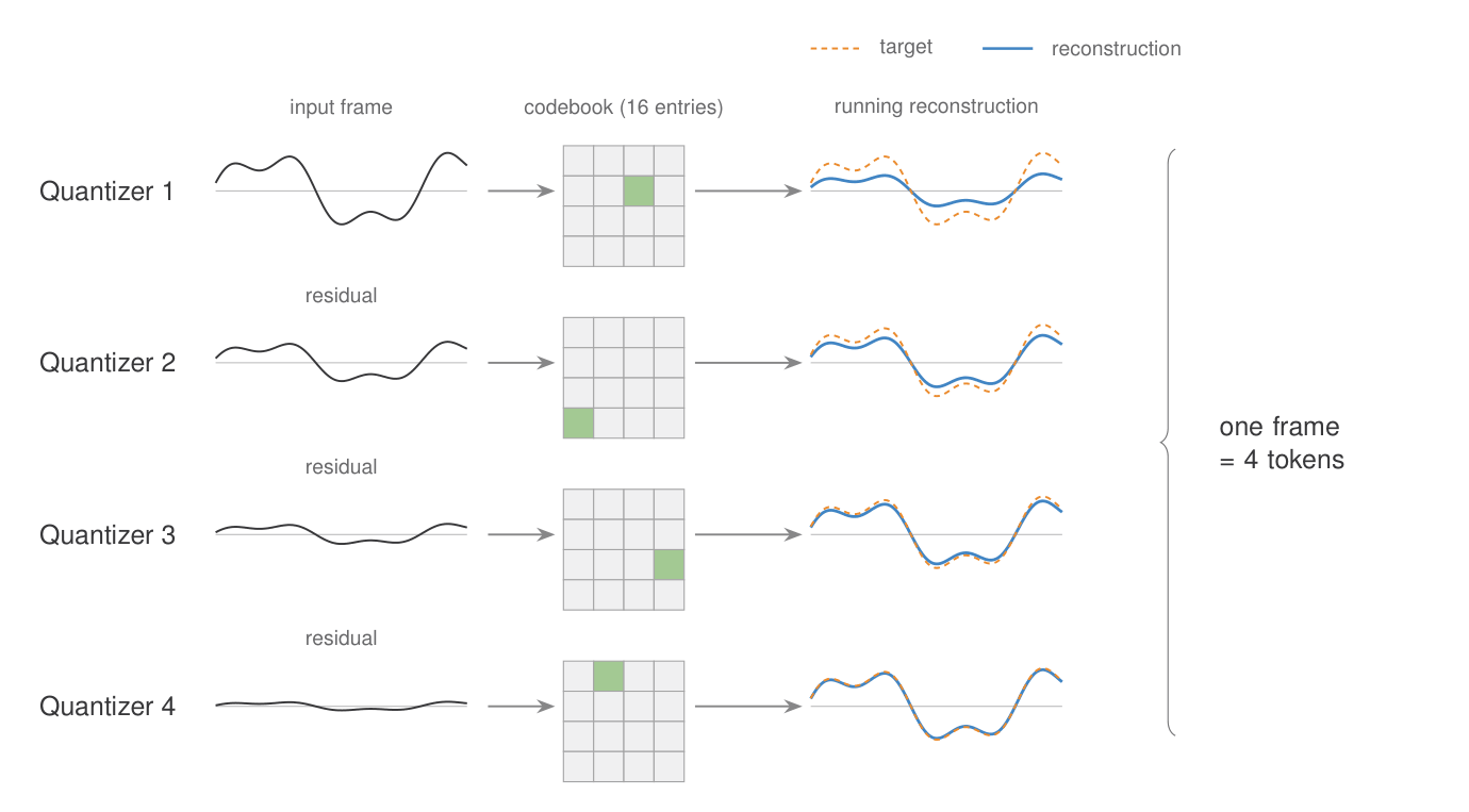
Figure 3 — Each quantizer encodes only the error the previous one left behind; four codebooks make one frame.

SoundStream (2021) put a fully convolutional encoder-decoder around an RVQ bottleneck and trained the whole thing end to end with adversarial and reconstruction losses together. The training trick that makes the truncation property real is structured dropout over quantizer layers: during training, a random number of quantizers is used, so the model learns to produce usable output at every depth. A single model spans 3 to 18 kbps with negligible quality loss against models trained at each fixed bitrate, and runs in real time on a smartphone CPU.

EnCodec (2022) followed the same blueprint with different engineering. A single multiscale spectrogram adversary replaces a more complex discriminator stack. A loss balancer redefines each loss weight as the fraction of total gradient it should contribute, decoupling the hyperparameter from the loss’s natural scale — a genuinely useful idea for any multi-objective training setup. And a lightweight Transformer can entropy-code the quantized units afterward for up to 40% further compression while staying faster than real time. EnCodec is what VALL-E tokenizes with.

w2v-BERT (2021) belongs here too, on the other side. It combines the contrastive objective and masked language modeling in one end-to-end model: the contrastive module learns to discretize the signal, and the MLM module learns contextualized representations by predicting those discrete tokens. Unlike HuBERT, no iterative re-clustering and re-training; unlike vq-wav2vec, not two separately trained modules bolted together. AudioLM uses w2v-BERT as its semantic tokenizer.

GSLM (2021) is the bridge between the two halves of this post. It established the template — a discrete speech encoder producing pseudo-text units, a language model trained over those units, a decoder turning units back into waveform — and showed you could learn the acoustic and linguistic characteristics of a language from raw audio with no text and no labels at all. It also surfaced the limitation that motivated everything after: semantic units alone give you coherent language in a single voice under clean conditions, and nothing else.

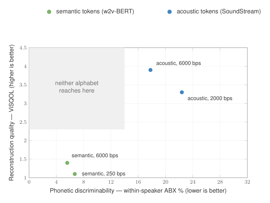
Figure 4 — Semantic and acoustic tokens are each worst at exactly what the other is best at.

Part two: generation

AudioLM (2022)

AudioLM’s contribution is a way to use both alphabets at once by ordering them: predict structure first, then predict sound conditioned on that structure.

The tokenizers. Semantic tokens come from an intermediate layer of the MLM module of w2v-BERT — a 0.6B-parameter Conformer — with k-means applied to those embeddings. Two specifics matter. The layer is the 7th, chosen empirically for phonetic discriminability. And the embeddings are normalized to zero mean and unit variance per dimension before clustering, which the authors report significantly improves discriminability. With K = 1024 clusters at 25 Hz, that’s 250 bps.

Acoustic tokens come from SoundStream at 50 Hz — a 320-fold reduction from 16 kHz — with N = 1024 entries per quantizer.

Notice the rate mismatch: SoundStream runs at twice w2v-BERT’s rate, so each semantic token spans two acoustic frames. Every stage of generation has to respect that 2:1 relationship.

Three stages, each a separate decoder-only Transformer trained on next-token prediction.

# AudioLM generation.
# Notice what's NOT here: no text, no transcript, no phonemes, anywhere.

def generate(prompt_audio):
    # Stage 1 — semantic. Long-term structure: what gets said.
    z = w2v_bert_tokens(prompt_audio)              # 25 Hz, K=1024
    z_hat = semantic_lm.generate(z)                # p(z_t | z_<t)

    # Stage 2 — coarse acoustic. Speaker, room, recording chain.
    # Conditioned on the ENTIRE semantic sequence, not just the past.
    y_coarse = coarse_lm.generate(
        condition=z_hat,
        history=soundstream_tokens(prompt_audio)[:, :Q_prime],
    )

    # Stage 3 — fine acoustic. Conditioned on coarse tokens only.
    # <-- semantic tokens are deliberately dropped here
    y_fine = fine_lm.generate(condition=y_coarse)

    return soundstream_decode(y_coarse, y_fine)

Two design choices in that structure repay attention.

Why the hierarchy is legal. It encodes a conditional independence assumption: semantic tokens are treated as independent of past acoustic tokens given past semantic tokens. Formally, p(z_t

z_<t, y_<t) ≈ p(z_t

z_<t). If that holds, you can factor generation into stages instead of modeling one giant interleaved sequence — which also keeps each stage’s sequence short enough to train.

Why stage 3 drops the semantic conditioning. The fine quantizers encode the residual left over after the coarse ones. That residual is fine acoustic texture, and it doesn’t depend on which words were spoken. Conditioning on semantics there would lengthen the context without adding information.

Within each stage, the token stack is flattened in row-major order — all Q quantizers for frame 1, then all Q for frame 2 — with an offset added per quantizer layer so that codeword 5 from quantizer 1 and codeword 5 from quantizer 2 get distinct indices.

What it does. Prompted with three seconds of speech from a speaker never seen during training, AudioLM continues in that speaker’s voice, prosody, and recording conditions — reverberation and background noise included — with no transcript, no speaker embedding, and no fine-tuning. Trained on piano recordings instead, it continues melodies coherently.

The ablation that justifies the whole design. Train on acoustic tokens alone, prompt with four seconds, and the recording conditions and speaker identity are preserved perfectly while the linguistic content degrades into babbling. The semantic stage isn’t an optimization. It is the only thing holding language together over long spans.

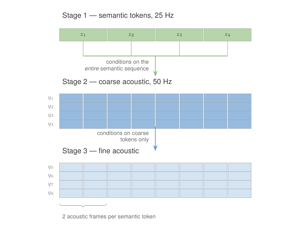
Figure 5 — Structure first, then sound: semantic tokens condition the coarse acoustics, which in turn condition the fine acoustics.

VALL-E (2023)

VALL-E reframes text-to-speech as conditional language modeling: condition on a phoneme sequence plus a three-second acoustic prompt from the target speaker, then predict the next acoustic token. Speaker adaptation becomes in-context learning — no speaker embedding, no per-speaker fine-tuning.

The architectural problem is the RVQ grid from the interlude. EnCodec gives VALL-E eight codebooks per frame at 75 Hz. Generating all eight autoregressively means 600 sequential forward passes per second of audio. Generating them all in parallel ignores that codebook 2 is defined as the residual after codebook 1.

The resolution is to split the grid along its two axes and use a different model for each:

# VALL-E: two Transformers, identical architecture, different attention masks.
# Both: 12 layers, 16 heads, d=1024, FFN 4096, dropout 0.1.

# AR model — codebook 1 only. Left-to-right, variable length.
# This is what decides how long the utterance is.
c1 = ar_model.generate(
    phonemes=phonemize(text),
    acoustic_prompt=encodec(reference_3s)[:, 0],    # first codebook only
)

# NAR model — codebooks 2..8. All time positions at once.
# Length is already fixed by c1, so nothing here needs sequential decoding.
# 7 forward passes total, not 7 x T.
codes = [c1]
for k in range(2, 9):
    codes.append(nar_model(
        phonemes=phonemize(text),
        acoustic_prompt=encodec(reference_3s),      # full stack
        previous=codes,                             # <-- residual ordering preserved
    ))

return encodec_decode(stack(codes))

The division of labour is the design. Everything sequential — duration, rhythm, where each word lands in time — is handled by the AR model over a single codebook. Everything parallel — acoustic refinement at positions whose timing is already settled — is handled by the NAR model. The residual ordering is preserved because codebook k is predicted conditioned on codebooks 1 through k−1.

Training data. 60k hours from Libri-Light. Since Libri-Light is unlabeled, the phoneme alignments came from a hybrid DNN-HMM ASR model trained on 960 hours of labeled LibriSpeech, decoding the unlabeled audio to best phoneme-level alignment paths at a 30 ms frameshift. EnCodec then produced the acoustic code matrix. Being able to train on 60k hours of non-studio audio is a direct consequence of the objective being next-token prediction rather than a synthesis loss demanding clean recordings.

A structural property worth understanding. Classical TTS architectures enforce monotonic alignment between text and audio — the synthesizer physically cannot skip a word, because the alignment mechanism advances through the input. A generic autoregressive language model has no such constraint. The authors report that words sometimes come out unclear, missed, or duplicated, and attribute it to disordered attention alignments in the AR phoneme-to-acoustic stage with nothing in the architecture preventing them. They also note weaker results on VCTK than LibriSpeech, reflecting limited coverage of accented speakers in audiobook data. This is a good illustration of what the language-modeling reframing costs: you inherit its generality and its scaling behaviour, and you give up the guarantees the special-purpose architecture provided for free.

Side by side

Model	Year	Frame rate	Discretization	Training objective	What it produces
wav2vec 2.0	2020	50 Hz	Product quantization, G=2 × V=320, Gumbel softmax	Contrastive over masked spans + diversity loss	Continuous contextual representations
HuBERT	2021	50 Hz	Offline k-means, 2 iterations, 100 → 500 clusters	Cross-entropy on masked frames only (α=1)	Semantic units
WavLM	2022	50 Hz	Inherits HuBERT’s	Masked prediction on mixed/noisy input, clean targets	Universal representations, speaker preserved
Whisper	2022	50 Hz	None on audio; BPE tokens on text out	Weakly-supervised seq2seq cross-entropy, 680k hrs	Text — transcription and X→En translation
SoundStream	2021	50 Hz	RVQ, structured quantizer dropout	Adversarial + reconstruction, end to end	Acoustic tokens, 3–18 kbps
EnCodec	2022	75 Hz	RVQ + optional entropy coding	Adversarial + reconstruction, loss balancer	Acoustic tokens
AudioLM	2022	25 + 50 Hz	w2v-BERT k-means + SoundStream RVQ	Next-token prediction, 3 stages	Speech and piano continuations
VALL-E	2023	75 Hz	EnCodec, 8 codebooks	Next-token (AR) + parallel prediction (NAR)	Zero-shot TTS from a 3s prompt

What is still open

No single alphabet does both jobs. The four numbers from Figure 4 haven’t been beaten by a representation that scores well on both axes at once. The workarounds are architectural — run two tokenizers and order them, or distill a semantic objective into a codec’s first codebook — rather than representational.

Sequence length remains the binding constraint. The trend is toward lower frame rates: 50 Hz for SoundStream, 25 Hz for AudioLM’s semantic tokens, and subsequent codecs have gone lower still. But each frame carries a stack, so the depth axis partly cancels the gains from the time axis.

Alignment has no principled home. Monotonic text-to-audio alignment was a structural guarantee in classical TTS and is a learned prior in codec language models. Recovering the guarantee without abandoning the language-modeling framing is unsolved.

Speaker and expression stay entangled. RVQ’s early codebooks bundle speaker identity, recording conditions and delivery together. That bundling is exactly what makes three-second voice cloning work, and exactly what makes independently controlling emotion without shifting perceived identity difficult.

The one-paragraph version

Speech has no natural vocabulary, so the first task in applying language models to audio was building one. Two research programs built two different alphabets. Self-supervised encoders — wav2vec 2.0 with a contrastive objective over product-quantized targets, HuBERT with cross-entropy over bootstrapped k-means labels, WavLM with the same scheme hardened against overlapping speakers — produce semantic tokens that capture linguistic content and reconstruct poorly. Neural codecs — SoundStream and EnCodec, both built on residual vector quantization — produce acoustic tokens that reconstruct faithfully and carry no long-range linguistic structure. AudioLM combined them hierarchically, generating semantic tokens first and conditioning coarse then fine acoustic tokens on them. VALL-E showed the codec’s token grid could be split along its two axes, with an autoregressive model handling timing over the first codebook and a non-autoregressive model refining the remaining seven in parallel, which turned zero-shot voice cloning into in-context learning from a three-second prompt. In both cases, the underlying move is the same: once audio is discrete, next-token prediction does the rest.

References

Foundations

1. van den Oord, A., Vinyals, O., & Kavukcuoglu, K. (2017). Neural Discrete Representation Learning (VQ-VAE). NeurIPS. arXiv:1711.00937. https://arxiv.org/abs/1711.00937 — origin of the learned discrete bottleneck everything here depends on.

Self-supervised encoders

1. Baevski, A., Zhou, H., Mohamed, A., & Auli, M. (2020). wav2vec 2.0: A Framework for Self-Supervised Learning of Speech Representations. NeurIPS. arXiv:2006.11477. https://arxiv.org/abs/2006.11477 — code and models: https://github.com/pytorch/fairseq

2. Hsu, W.-N., Bolte, B., Tsai, Y.-H. H., Lakhotia, K., Salakhutdinov, R., & Mohamed, A. (2021). HuBERT: Self-Supervised Speech Representation Learning by Masked Prediction of Hidden Units. IEEE/ACM TASLP, 29:3451–3460. arXiv:2106.07447. https://arxiv.org/abs/2106.07447

3. Chung, Y.-A., Zhang, Y., Han, W., Chiu, C.-C., Qin, J., Pang, R., & Wu, Y. (2021). w2v-BERT: Combining Contrastive Learning and Masked Language Modeling for Self-Supervised Speech Pre-Training. IEEE ASRU, 244–250. arXiv:2108.06209. https://arxiv.org/abs/2108.06209 — AudioLM’s semantic tokenizer.

4. Chen, S., Wang, C., Chen, Z., Wu, Y., Liu, S., Chen, Z., Li, J., Kanda, N., Yoshioka, T., Xiao, X., Wu, J., Zhou, L., Ren, S., Qian, Y., Qian, Y., Wu, J., Zeng, M., Yu, D., & Wei, F. (2022). WavLM: Large-Scale Self-Supervised Pre-Training for Full Stack Speech Processing. IEEE J-STSP, 16(6):1505–1518. arXiv:2110.13900. https://arxiv.org/abs/2110.13900 — models: https://aka.ms/wavlm

Weakly-supervised recognition

1. Radford, A., Kim, J. W., Xu, T., Brockman, G., McLeavey, C., & Sutskever, I. (2022). Robust Speech Recognition via Large-Scale Weak Supervision (Whisper). ICML 2023, PMLR 202:28492–28518. arXiv:2212.04356. https://arxiv.org/abs/2212.04356 — code and models: https://github.com/openai/whisper — the weak-supervision counterpoint to the self-supervised encoders.

Neural audio codecs

1. Zeghidour, N., Luebs, A., Omran, A., Skoglund, J., & Tagliasacchi, M. (2021). SoundStream: An End-to-End Neural Audio Codec. IEEE/ACM TASLP, 30:495–507. arXiv:2107.03312. https://arxiv.org/abs/2107.03312

2. Défossez, A., Copet, J., Synnaeve, G., & Adi, Y. (2022). High Fidelity Neural Audio Compression (EnCodec). TMLR. arXiv:2210.13438. https://arxiv.org/abs/2210.13438 — code: https://github.com/facebookresearch/encodec

Generative speech models

1. Lakhotia, K., Kharitonov, E., Hsu, W.-N., Adi, Y., Polyak, A., Bolte, B., Nguyen, T.-A., Copet, J., Baevski, A., Mohamed, A., & Dupoux, E. (2021). On Generative Spoken Language Modeling from Raw Audio (GSLM). TACL, 9:1336–1354. arXiv:2102.01192. https://aclanthology.org/2021.tacl-1.79/ — the first end-to-end textless pipeline.

2. Borsos, Z., Marinier, R., Vincent, D., Kharitonov, E., Pietquin, O., Sharifi, M., Roblek, D., Teboul, O., Grangier, D., Tagliasacchi, M., & Zeghidour, N. (2023). AudioLM: a Language Modeling Approach to Audio Generation. IEEE/ACM TASLP. arXiv:2209.03143. https://arxiv.org/abs/2209.03143 — samples: https://google-research.github.io/seanet/audiolm/examples

3. Wang, C., Chen, S., Wu, Y., Zhang, Z., Zhou, L., Liu, S., Chen, Z., Liu, Y., Wang, H., Li, J., He, L., Zhao, S., & Wei, F. (2023). Neural Codec Language Models are Zero-Shot Text to Speech Synthesizers (VALL-E). arXiv:2301.02111. https://arxiv.org/abs/2301.02111 — later published in IEEE TASLP, 33:705–718 (2025).

The code blocks in this post are illustrative pseudocode meant to expose architectural intent, not runnable implementations.