The Gatekeeper of Voice AI: A Deep Dive into Voice Activity Detection
Talk to any modern conversational AI, and you will notice a distinct rhythm. You speak, you pause, and almost instantly, the AI responds. The architecture enabling this fluid interaction isn’t just the multi-billion parameter speech-to-text transcription engine. It is a much smaller, microsecond-latency system sitting at the very edge of the microphone, deciding whether you have stopped talking or just paused to take a breath.
This is the Voice Activity Detection (VAD) module.
A VAD module is a binary gatekeeper. It chops a continuous audio stream into tiny slices and decides, millisecond by millisecond, whether to pass that audio to heavy, expensive downstream models or to drop it entirely. Without it, Automatic Speech Recognition (ASR) models would waste massive amounts of compute trying to transcribe air conditioning hums and keyboard clicks.
The Vocabulary of VAD
Before analyzing the architectures, we must define the primitives of real-time audio processing:
- Framing: Real-time audio processing does not evaluate whole sentences. The continuous signal is windowed into non-overlapping or overlapping frames, typically 10 ms to 30 ms long.
- Hangover (Holdover): Natural speech contains tiny silences that are not pauses at all. A plosive like “p” or “t” is produced by sealing the vocal tract, so its closure phase is genuine acoustic silence in the middle of a word. Phoneticians studying conversational timing bridge silences shorter than roughly 180 ms precisely to avoid mistaking these closures for pauses [6]. A hangover mechanism does the same thing for a VAD: it holds the “speech detected” state for a number of frames after the signal goes quiet, preventing utterance truncation. It is also a latency floor you cannot optimize away.
- Likelihood Ratio Test (LRT): A statistical hypothesis test used to compare the goodness of fit of two competing models (e.g., a speech model vs. a noise model).
- Mel-Spectrogram: A visual representation of the spectrum of frequencies of a signal as it varies with time, mapped to the Mel scale to mimic human ear perception.
The Core Idea
A VAD module is fundamentally an information bottleneck that decides what constitutes “signal” versus “noise.” The evolution of VAD is not just about writing better code; it is entirely about finding better mathematical representations of that signal. Over the past twenty years, researchers have placed three distinct bets on how to separate human speech from everything else.
The Amplitude Bet: Time-Domain Heuristics
The earliest approach to VAD assumes that when someone speaks, the signal’s physical properties change in obvious, measurable ways compared to background room tone.
This approach relies on extracting time-domain features, primarily Root Mean Square (RMS) Energy and the Zero-Crossing Rate (ZCR). Voiced speech (like vowels) carries high energy, while unvoiced speech (like the “s” sound) has low energy but crosses the zero-amplitude axis very frequently due to its high-frequency nature.
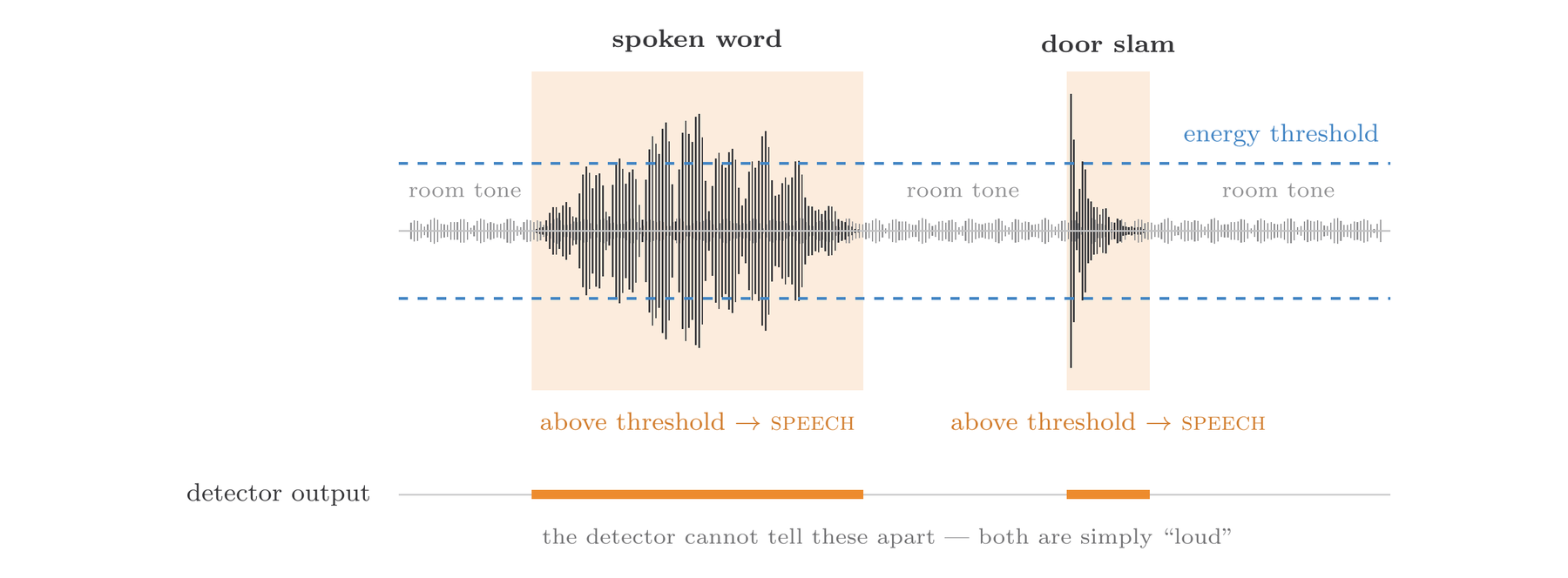
Figure 1 — The energy thresholding failure mode. A static threshold cannot distinguish a spoken word from a door slam, because it only measures loudness.
def is_speech_heuristic(frame, energy_thresh, zcr_thresh):
    # Calculate RMS Energy
    energy = np.sqrt(np.mean(np.square(frame)))

    # Calculate Zero-Crossing Rate
    crossings = np.sum(np.abs(np.diff(np.sign(frame)))) / (2 * len(frame))

    # <-- The fatal flaw: static thresholds fail when SNR drops
    if energy > energy_thresh or crossings > zcr_thresh:
        return True
    return False
While computationally nearly free, static thresholds are mathematically brittle. If you tune the threshold for a quiet laboratory, the system will trigger endlessly in a coffee shop.
The Statistical Bet: WebRTC VAD
Time-domain amplitude proved insufficient for robust Voice over IP (VoIP). Instead of betting on amplitude, the WebRTC detector bets on statistical frequency distributions across the band where the human vocal tract puts most of its power.
The standard-bearer for this approach is the open-source WebRTC VAD. It operates on a decision-theoretic framework. For a given audio frame, it evaluates two hypotheses:
- H₀: The frame contains only noise.
- H₁: The frame contains speech (and possibly noise).
WebRTC splits the incoming frame into six sub-bands spanning roughly 80 Hz to 4 kHz and models the distribution of speech and noise in each band with a two-component Gaussian mixture. For each band it computes a log-likelihood ratio between the two hypotheses. The 4 kHz ceiling is not a claim about where speech ends — it follows from the fact that the detector runs internally at 8 kHz, downsampling 16, 32 and 48 kHz inputs before it ever sees them. It is a telephone-band model in the literal sense.
The detail that most descriptions omit is how those six ratios are combined. They feed two separate tests: a spectrum-weighted sum compared against a global threshold, and each individual ratio compared against a local threshold. In the source, the two are OR’d — a single band clearing its local threshold is sufficient to declare speech. That bias toward firing is deliberate, and it comes straight from the telephony setting the detector was designed for, where a clipped syllable costs more than a wasted packet.
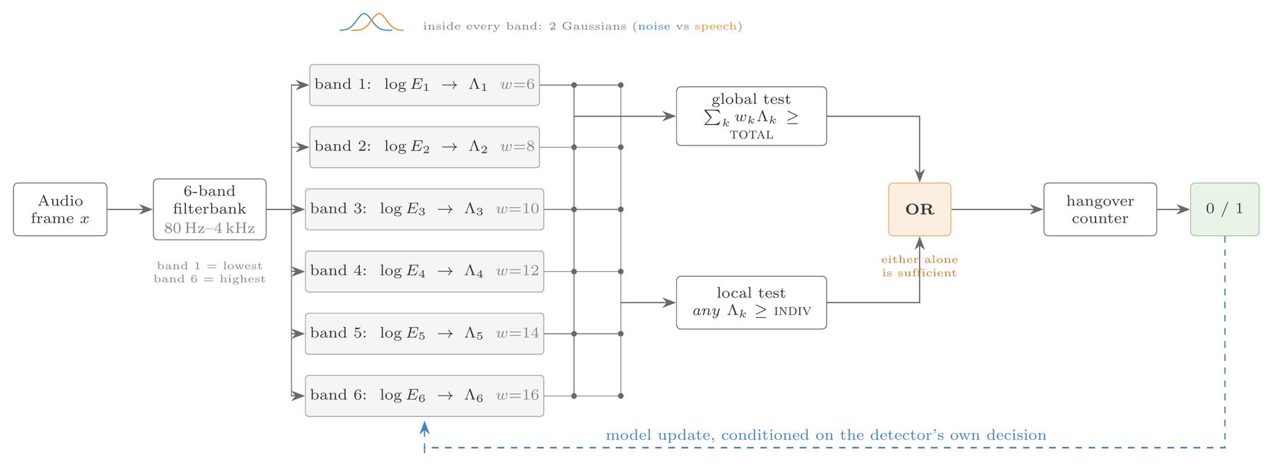
Figure 2 — The statistical sub-band architecture of WebRTC VAD. Six bands, two Gaussians each, and two tests that are OR’d rather than combined. The dashed path is the online adaptation loop.
WebRTC VAD remains a gold standard for real-time edge devices because the whole model is a few hundred bytes and evaluates in microseconds. The static tables compiled into vad_core.c are only the initial parameters, though: at runtime the detector updates its noise means when it decides a frame is noise, and its speech means when it decides a frame is speech. It trains itself on its own output, with no labels anywhere in the loop — which is exactly what you want on a long call with a drifting noise floor, and also self-reinforcing enough that the implementation carries explicit guards to stop the two models from collapsing into each other.
The deeper catch is that the GMM evaluates each frame in near-isolation. A sudden, sharp noise that overlaps with vocal frequencies — a siren, a squeaking chair — will instantly fool the model because it lacks any temporal context.
The Context Bet: Deep Learning and Transformers
Modern architectures abandon hand-crafted statistical filters. Instead, they frame VAD as a sequence modelling problem.
They bet that you cannot confidently classify a 30 ms slice of audio without knowing what happened 500 ms ago. A neural network can look at the surrounding sequence and recognize an isolated loud pop as noise, not a phoneme.
Silero VAD is the production workhorse of this generation, and it is remarkably small: independent ports of the v5 checkpoint put it at roughly 309 thousand parameters, running on 512-sample chunks (32 ms at 16 kHz) with LSTM state carried from one chunk to the next. That carried state is the entire difference from a GMM. The door slam no longer becomes a speech onset, because the recurrent state knows nothing speech-like preceded it.
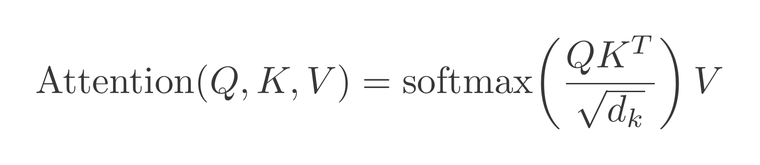
Transformer-based VADs go further, projecting Mel-spectrogram patches into a continuous embedding space and applying multi-head self-attention, so the network can dynamically weigh the importance of past and future frames:
class TransformerVAD(nn.Module):
    def forward(self, mel_spectrogram_sequence):
        # Expected input: A sequence of frames capturing ~1 second of context
        # Project 80-bin Mel features to the Transformer dimension
        x = self.input_projection(mel_spectrogram_sequence)

        # Self-attention evaluates global context, decoupling transient
        # noise from sustained vocal cord resonance.
        x = self.transformer_encoder(x)

        # Output a probability for each frame
        logits = self.classifier(x)
        return torch.sigmoid(logits)
By leveraging self-supervised speech foundation models fine-tuned with linear classification heads, these models achieve exceptional boundary detection in highly degraded audio environments.
Side by Side
| Architecture | Signal Representation | Temporal Context | Latency | Compute Complexity |
|---|---|---|---|---|
| Time-Domain (ZCR/Energy) | Raw audio amplitude | None (10 ms isolated) | Ultra-low (<1 ms) | O(N) |
| WebRTC VAD (GMM) | 6 sub-band log-energies | None (relies on hangover) | Low (~10 ms) | Low (a few hundred bytes) |
| Silero VAD (CNN/RNN) | Learnable filterbanks | Implicit (LSTM hidden state) | Medium (32 ms chunks) | Low (~309K params) |
| Transformer VAD (AST) | Mel-spectrogram patches | Explicit (self-attention) | High (requires sequence) | High (10M+ params) |
What is still hard
If you are preparing to implement a VAD in production or discuss it in a system design interview, you must understand where the abstractions leak:
The Receiver Operating Characteristic (ROC) Reality: VAD is a tradeoff between False Positives (waking up for noise) and False Negatives (clipping the user’s speech). In production, you almost always bias toward accepting false positives. It is slightly cheaper to process 100 ms of a door slamming than it is to accidentally cut off the first syllable of the user’s query and ruin the transcript. Report the curve rather than a single accuracy number: a detector can be right about 95% of frames and still shatter every utterance into fragments, which is why event-level boundary scores belong alongside frame-level ones.
Babble noise: The hardest test for any VAD is a crowded room where multiple people are talking in the background. A VAD’s job is to detect “human speech.” If it successfully ignores the air conditioning but triggers when the person at the next table orders a coffee, the algorithmic math worked, but the product failed.
The fix is not a better VAD — it is a different question. Personal VAD [7] reframes the task as three-class rather than binary: non-speech, non-target speaker, and target speaker, conditioning the network on a d-vector speaker embedding computed once during an enrollment step. Target-Speaker VAD [8] goes further, estimating speaker embeddings from the recording itself rather than requiring enrollment, and predicting every speaker’s activity jointly, which is why it dominates diarization on overlapped meeting audio. If your agent runs anywhere other than a headset, this is the family you want, and the cost is an extra embedding model in the hot path rather than heavyweight offline diarization.
The Latency vs. Context tradeoff: Transformers are highly accurate because they evaluate sequence context. But you cannot evaluate context without waiting for future frames to arrive. If a model needs 300 ms of future audio to confidently classify the current frame, you have permanently injected a 300 ms delay into the conversational loop. This is worth separating from compute cost: algorithmic latency is how much future audio the model requires, while real-time factor is how fast inference runs, and a model can be fast and still unusable live. Human turn-taking sets the bar unforgivingly — median gaps between turns sit around 100 ms, with cross-linguistic medians between 0 and 300 ms [6]. Against that, a bidirectional model over a long window is not slow. It is disqualified.
The one paragraph version
A Voice Activity Detection (VAD) module is a gating mechanism that filters silence and background noise out of continuous audio streams to save downstream compute. Early systems relied on time-domain volume thresholds, which proved brittle in noisy environments. Statistical models like WebRTC VAD solved this by evaluating frequency sub-bands against Gaussian mixtures whose parameters adapt online, becoming the standard for low-latency VoIP. Today, deep learning models like Silero and Transformer-based VADs treat audio as sequential contexts, using recurrent layers and self-attention to separate human speech from complex ambient noise, though they force engineers to carefully balance precision against real-time latency.
References
- Sohn, J., Kim, N. S., & Sung, W. (1999). A statistical model-based voice activity detection. IEEE Signal Processing Letters, 6(1), 1–3. — The foundational paper establishing the Likelihood Ratio Test for VAD.
- WebRTC Project.
common_audio/vad/vad_core.c. C source for the sub-band GMM detector, including the OR’d global and local tests and the online mean updates. https://github.com/wiseman/py-webrtcvad/blob/master/cbits/webrtc/common_audio/vad/vad_core.c - Wiseman, J. py-webrtcvad. Python bindings for the WebRTC detector. https://github.com/wiseman/py-webrtcvad
- Silero Team. Silero VAD: pre-trained enterprise-grade Voice Activity Detector. GitHub repository. https://github.com/snakers4/silero-vad — MIT licensed; note that the training data and full architecture are not publicly disclosed.
- Gong, Y., Chung, Y., & Glass, J. (2021). AST: Audio Spectrogram Transformer. Interspeech 2021. arXiv:2104.01778. https://arxiv.org/abs/2104.01778
- Heldner, M., & Edlund, J. (2010). Pauses, gaps and overlaps in conversations. Journal of Phonetics, 38(4), 555–568. — Source of the ~100 ms median turn gap and the 180 ms stop-closure bridging threshold.
- Ding, S., Wang, Q., Chang, S.-Y., Wan, L., & Moreno, I. L. (2020). Personal VAD: Speaker-Conditioned Voice Activity Detection. Odyssey 2020. — The three-class formulation with d-vector enrollment.
- Medennikov, I., et al. (2020). Target-Speaker Voice Activity Detection: a Novel Approach for Multi-Speaker Diarization in a Dinner Party Scenario. Interspeech 2020. arXiv:2005.07272. https://arxiv.org/abs/2005.07272
- Chaudhuri, S., Roth, J., Ellis, D. P. W., et al. (2018). AVA-Speech: A Densely Labeled Dataset of Speech Activity in Movies. Interspeech 2018. arXiv:1808.00606. https://arxiv.org/abs/1808.00606 — A shared benchmark, scoring clean speech, speech-over-music and speech-over-noise separately.
The code in this post is illustrative pseudocode meant to expose intent, not runnable implementations. For working code, see the linked repositories.