How Audio Becomes Tokens

Part two. Last time I explained why full-duplex models predict the next 80 milliseconds of their own audio stream. My friend’s follow-up was the right one: “okay, but what IS 80 milliseconds of audio to a transformer?”

---

Starting from the actual beginning

A language model doesn’t see words. It sees integers.

When you type “hello” into an LLM, a tokenizer converts it to something like [15496], the model looks up row 15496 of a big table of vectors, and everything after that is arithmetic on numbers. When it answers, it produces a probability distribution over its vocabulary — maybe 50,000 possible next tokens — samples one, and looks up what text that integer means.

This works because text was already made of symbols before anyone built a computer. Letters and words are discrete things. A tokenizer just regroups symbols that already exist.

Audio has no symbols in it. Audio is air pressure, measured 24,000 times a second, stored as a long list of numbers like [0.021, -0.014, 0.008, ...]. There is no point in that list where one “unit” ends and another begins. There’s no vocabulary. There’s nothing to look up.

So before a full-duplex model can predict anything, something has to invent a vocabulary for sound — and then be able to turn sequences from that vocabulary back into audio you’d actually want to listen to.

That something is a neural audio codec. This post is about how it works, where the idea came from, and why the specific design used by models like Moshi looks the way it does.

I’m going to build it up from the bottom. If you already know what RVQ is, skip to “The two families.”

---

Part 1: What a codec is

“Codec” is a portmanteau of coder and decoder. It’s any pair of programs where one squeezes data down for storage or transmission, and the other expands it back out. MP3 is a codec. JPEG is a codec. The thing making your voice fit down a phone line is a codec.

Almost all the interesting ones are lossy: the output isn’t identical to the input. You accept that in exchange for the file being twenty times smaller, and the trick is throwing away the parts people won’t notice are missing. MP3 discards frequencies masked by louder nearby sounds, because human hearing can’t detect them anyway.

Here’s the number that motivates everything: raw CD-style audio runs at hundreds of kilobits per second. A 1990s cell phone had to work in about 10. That’s not a compression problem you solve by being clever with redundancy. You need a fundamentally different approach.

The 1939 idea that still runs everything

In 1939, Homer Dudley at Bell Labs demonstrated the Vocoder — short for voice coder. His insight is the one this entire field still rests on:

Don’t transmit the sound. Transmit a description of how to make the sound, and rebuild it at the other end.

Human speech isn’t arbitrary noise. It’s produced by a physical system: vocal cords vibrating at some pitch, air passing through a throat and mouth shaped in particular ways. So instead of sending the waveform, send a handful of parameters — pitch, loudness, the rough shape of the vocal tract — and have the receiver synthesize fresh speech from those parameters.

The bandwidth saving is enormous, because you’ve stopped sending audio and started sending instructions.

This split has a name that persists today. The part that extracts parameters is the analyzer (encoder). The part that rebuilds sound from them is the synthesizer — and in modern speech AI, the component that turns compact representations back into waveforms is still called a vocoder. Same word, eighty-odd years later.

Everything from 1970s Linear Predictive Coding through the codecs in every cell phone is a refinement of this: build a mathematical model of how speech is produced, send the model’s parameters.

Where classical codecs hit a wall

That approach has a ceiling, and the ceiling is the model.

Push a classical parametric coder down to around 2.4 kbps and the speech is intelligible but unmistakably robotic. Not because 2.4 kbps is too few bits — as we’ll see, it isn’t — but because a hand-designed model of the human vocal tract is a crude approximation. Real speech contains texture the equations don’t capture, and what the model can’t describe, it can’t transmit.

The obvious fix: stop hand-designing the model. Learn it.

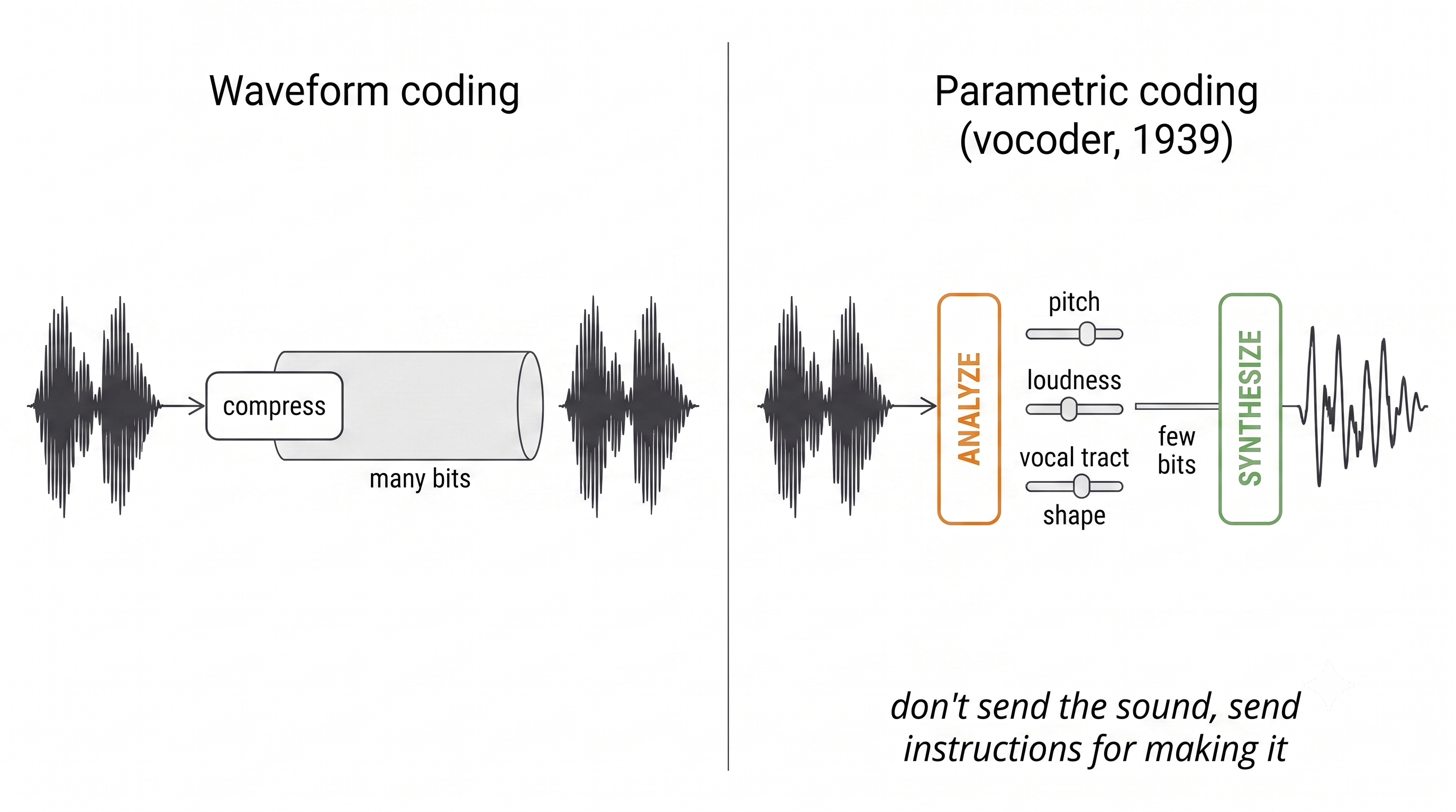
Figure 1 - The 1939 idea. Don’t send the sound, send instructions for making it.

---

Part 2: Why “compressed” isn’t enough

Before the history, one thing worth settling, because it trips people up.

MP3 already compresses audio into a small number of bits. Why can’t a language model just use MP3 bits as its tokens?

Because a compressed bitstream and a vocabulary are different kinds of object.

An MP3 bitstream is a densely packed sequence where meaning depends on position and context. Flip one bit and you may corrupt everything after it. There’s no sense in which “bit pattern 0110” is similar to “bit pattern 0111” — nearby codes don’t mean nearby sounds.

A language model needs something much more specific:

• A fixed, finite vocabulary. The output layer is a softmax over N options; N has to be a manageable number and it can’t change.
• Meaningful units. Each token should stand for something coherent, so that similar tokens can get similar embeddings and the model can generalize across them.
• Sampleability. Generation means drawing from a probability distribution over the vocabulary. You can’t sample from “the next 400 bits of an MP3 stream” in any useful way.

So the job isn’t compression. It’s compression into a vocabulary: a fixed set of learned sound-units where nearby units mean similar sounds, and any sequence of them decodes to plausible audio.

That’s a strictly harder problem than MP3 was solving, and it’s why neural audio codecs are their own field.

---

Part 3: A brief history, in two families

The confusing thing about this area — and the reason “semantic tokens” and “acoustic tokens” both exist — is that two completely separate research lineages developed discrete representations of speech for completely different reasons, and only merged around 2022.

Family A: the compression lineage

Goal: make it small, then rebuild it faithfully.

2016 — WaveNet. DeepMind trained a neural network to generate raw audio one sample at a time, predicting each of the 24,000-per-second values from the ones before it. It sounded dramatically better than anything parametric. It was also far too slow for real time — 24,000 sequential forward passes per second of audio.

But it changed the question. If a network can synthesize convincing speech from a compact conditioning signal, then the encoder no longer has to preserve the waveform. It only has to preserve enough for the decoder to imagine a plausible one. That’s Dudley’s 1939 insight with a learned synthesizer instead of a hand-built one.

2017 — VQ-VAE. An autoencoder is a network that squeezes input through a narrow middle layer and reconstructs it; the middle layer (the “latent”) is a compact continuous vector. VQ-VAE added one thing: force that latent to be one of a finite learned set of vectors — a codebook. Now the middle of your autoencoder is an integer. This is where audio tokens actually begin.

2018–2019 — the two get combined. Kleijn and colleagues at Google put a WaveNet decoder on a 2.4 kbps parametric bitstream. Then Gârbacea and colleagues built a VQ-VAE with a WaveNet decoder running at 1.6 kbps with quality between a 2.4 kbps classical codec and a 23 kbps one. A learned encoder producing discrete codes, a learned decoder producing audio — the shape of everything since.

2021 — SoundStream. Google’s fully end-to-end neural codec, trained adversarially, streaming, and introducing residual vector quantization as the workhorse (Part 5). 2022 — EnCodec from Meta refined the recipe.

By 2022 you could turn speech into discrete tokens and back with good quality at very low bitrates. These are acoustic tokens: optimized to reconstruct.

Family B: the understanding lineage

Goal: learn what speech means, with no interest in reconstructing it.

Entirely different motivation. Speech recognition needs labeled data, labeled data is expensive, so researchers built self-supervised models that learn from raw audio with no transcripts by predicting masked-out portions of their own input — the same trick that made BERT work for text.

wav2vec 2.0 (2020), HuBERT (2021), and WavLM (2022) came out of this. Their hidden representations turn out to encode phonetic content remarkably well: fine-tune them and you get strong ASR, speaker identification, emotion recognition.

Cluster or quantize those hidden states and you get discrete units too. But these are semantic tokens: they track what was said. They deliberately discard speaker identity, pitch, and room acoustics, because those are nuisance variables for recognition.

The collision

Two families, two kinds of token, and around 2022 people trying to build speech language models discovered an annoying fact:

• Train an LM on acoustic tokens and it generates audio that sounds like speech but means nothing. Fidelity without content.
• Train an LM on semantic tokens and it produces sensible content you can’t turn into good audio, because the information needed to synthesize was thrown away. Content without fidelity.

AudioLM (2022) resolved this by using both, in stages: model semantic tokens first to get the content right, then generate acoustic tokens conditioned on them.

SpeechTokenizer (2023) asked the better question — why two token sets? — and made a single RVQ codec where the first level is trained to match a self-supervised model’s representation, so level one carries meaning and the rest carry sound.

Mimi (2024), the codec inside Moshi, takes that and adds what full-duplex specifically needs: fully streaming operation, a frame rate chosen to sit near text, and a structural fix to a problem SpeechTokenizer’s approach creates. That’s Part 7.

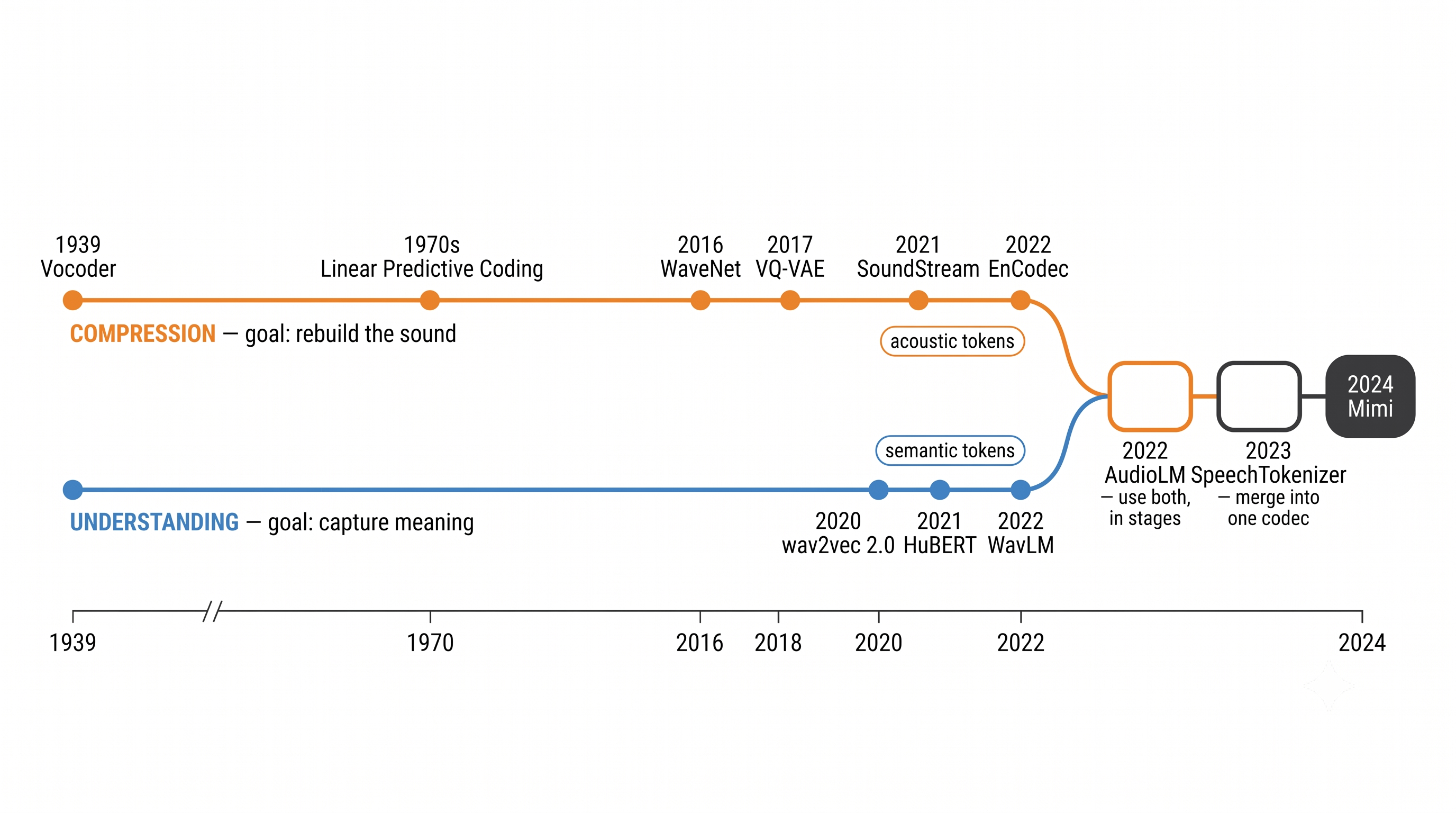
Figure 2 - Two research lineages, converging. Compression wanted fidelity; understanding wanted meaning.

---

Part 4: Vector quantization, from scratch

Now the mechanism. It’s simpler than the acronyms suggest.

Imagine you want to describe a photograph using only the 120 colors in a big box of crayons. For each region, you find the crayon closest to the actual color and write down its number. To rebuild the picture, someone looks up crayon 47 and colors it in.

You’ve just done vector quantization. The crayon box is a codebook. Each crayon is a codeword. “Find the closest one” is the encoder; “look up the number” is the decoder.

Now two changes to make it useful for audio.

The things being matched aren’t colors, they’re chunks of sound. The encoder — a convolutional network — reads a short slice of waveform and produces a vector of, say, 256 numbers summarizing it. That vector is what gets matched.

The crayon box is learned, not given. This matters more than it sounds. A generic box wastes most of its crayons on colors the photo never uses. A codebook trained on speech puts its entries exactly where speech actually lives — clustered around real phonetic and acoustic configurations. Every entry earns its place.

In code, encoding is one line of arithmetic:

def vq_encode(z, codebook):
    """z: one 256-number summary of a chunk of sound.
       codebook: (K, 256) -- our K learned 'crayons'.
       Returns: which crayon is closest."""
    distances = ((codebook - z) ** 2).sum(axis=1)   # distance to every entry
    return distances.argmin()                        # nearest one wins

def vq_decode(index, codebook):
    """Look up the crayon."""
    return codebook[index]

That’s it. The encoder outputs an integer. The decoder looks it up.

One practical wrinkle worth knowing, because it explains an implementation detail you’ll see everywhere: codebook collapse. If some entries never win, they never get updated, so they never improve, so they never win — a chunk of your vocabulary dies unused. Codecs fight this by maintaining entries as running averages of the vectors assigned to them and by resetting dead entries to live encoder outputs.

---

Part 5: The wall, and residual vector quantization

Here’s the problem that RVQ exists to solve. I want to build it up before writing any numbers, because the numbers only land once you feel the shape.

How many crayons do you need?

Speech is not simple. Every combination of phoneme, pitch, speaker, loudness, and room acoustic is a different sound. If one codebook entry must capture a whole chunk of speech in one lookup, you need an entry for every meaningfully different combination.

Think about describing paint colors. You could maintain a catalog with a unique name for every distinguishable shade — but there are millions, and the catalog is useless. Or you could say “red, plus a bit of blue, plus a touch of white.” A handful of primaries, combined, covering the whole space.

Vector quantization as described so far is the catalog. It needs a unique entry per distinguishable sound, and that number is astronomically large.

The fix is to describe in layers.

Guess roughly. Look at how wrong you were. Guess the correction from a second codebook. Look at what’s still wrong. Guess again. Each stage only has to describe the leftover error — the residual — from the stage before.

It’s how you’d sketch: rough shapes first, then refine, then detail. Or how a progressive JPEG loads — blurry, then sharper, then sharp.

That’s residual vector quantization, and the code is startlingly short:

def rvq_encode(z, codebooks):
    """Describe z in layers, coarse to fine."""
    residual = z              # what we still need to explain
    indices  = []
    for cb in codebooks:
        i = vq_encode(residual, cb)     # best guess at what's left
        indices.append(i)
        residual = residual - cb[i]     # subtract it; keep the leftover
    return indices                       # one integer per layer

def rvq_decode(indices, codebooks):
    """Add the layers back up. That's the entire decoder."""
    return sum(cb[i] for i, cb in zip(indices, codebooks))

Look at rvq_decode: reconstruction is just a sum. Layer one gives the rough shape, layer two adds a correction, layer eight adds a fine detail. Stack them and you get the original back.

Now the numbers

With the intuition in place, the arithmetic is where it becomes obvious why this won.

Mimi uses 8 layers, each with a codebook of 2,048 entries. Picking one of 2,048 options takes 11 bits (2¹¹ = 2,048), so a frame of audio costs 8 × 11 = 88 bits.

Ask what a single codebook would need to express those same 88 bits. It would need one entry for every distinct 88-bit pattern:

2⁸⁸ ≈ 310,000,000,000,000,000,000,000,000 entries.

You cannot store that. You cannot search it. You could never train it — you’d need to encounter each entry many times.

What does RVQ store instead?

8 × 2,048 = 16,384 vectors. A small matrix.

Same expressive range. Sixteen thousand vectors instead of 3 × 10²⁶. The layered structure converts a multiplicative explosion into an additive cost — and that single fact is why discrete audio tokens are practical at all. Every neural audio codec since SoundStream uses this.

One nice bonus: because the layers are ordered coarse-to-fine and decoding is just addition, you can stop early. Use three layers instead of eight and you get valid audio, just rougher. Mimi is trained with up to 32 layers and runs with 8 — the operating point where quality is good enough and the language model still only has to predict 8 numbers per frame.

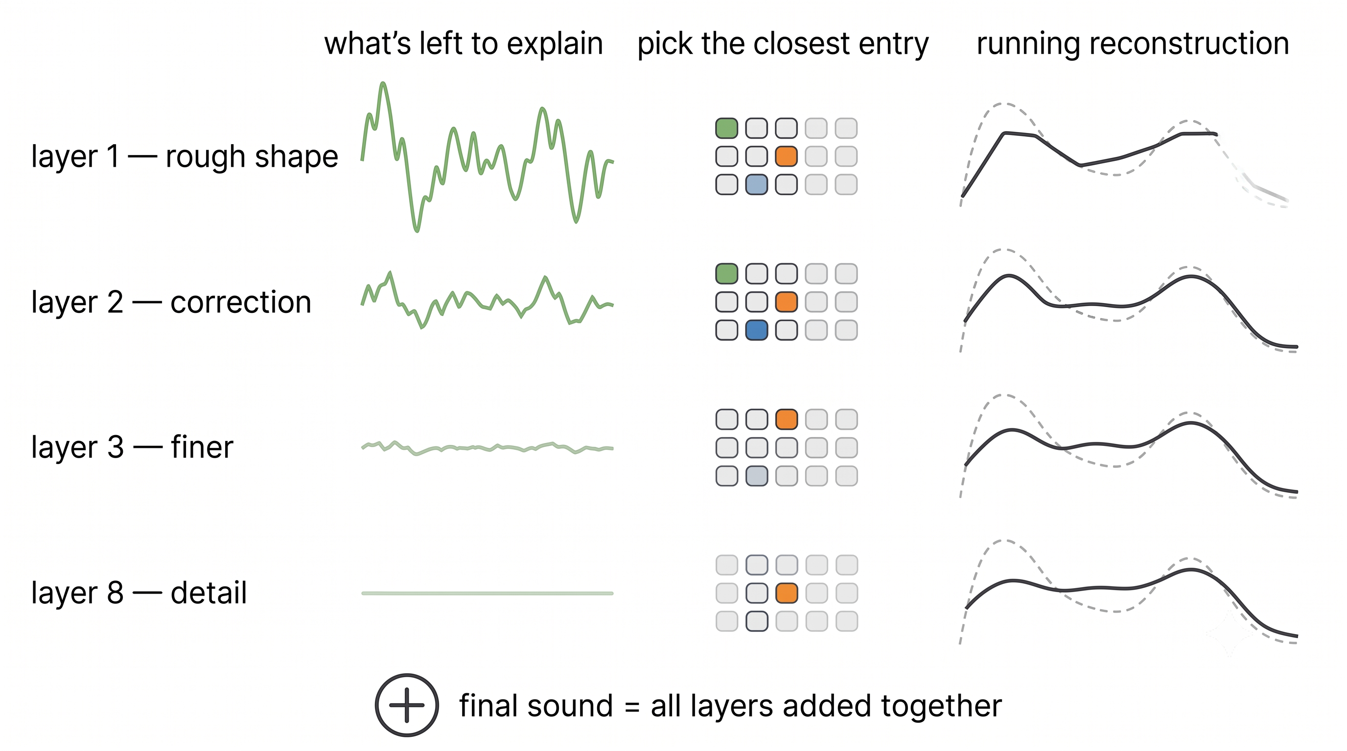
Figure 3 - Describing sound in layers. Each layer only encodes the error left by the one before.

---

Part 6: Wait — 88 bits is nothing

Worth pausing on, because it’s genuinely surprising.

88 bits per 80ms frame, 12.5 frames per second, works out to 1.1 kilobits per second. Raw 24kHz 16-bit audio is 384 kbps. That’s roughly 350× compression — and it still sounds like a person.

Recall that classical parametric codecs sounded robotic at 2.4 kbps, more than twice this bitrate.

How? Because of what changed in 2016. The decoder is no longer applying a hand-built vocal-tract model — it’s a trained neural network that has heard millions of hours of speech and has extremely strong priors about what human speech sounds like. It doesn’t need to be told the fine texture of a voice. It only needs enough of a hint to generate texture that’s plausible.

This shows up directly in how Mimi is trained. Rather than asking the decoder to match the original waveform, it’s trained adversarially — a discriminator network tries to tell Mimi’s output from real speech, and Mimi tries to fool it. At 1.1 kbps faithful reconstruction is impossible in principle; there aren’t enough bits. So don’t optimize for accuracy. Optimize for believability.

The decoder isn’t decompressing. It’s imagining, with constraints.

---

Part 7: Mimi, and the problem it fixes

Now we can look at the actual codec inside Moshi, and every piece should feel motivated.

The frame rate is a language-modeling decision

Mimi turns 24kHz audio into 12.5 frames per second — one frame every 80 milliseconds, 1,920 samples.

Earlier codecs ran at 50 or 75 frames per second. Mimi went much lower, and the reason has nothing to do with audio quality:

Text tokens arrive at about 3–4 per second in normal speech. At 12.5 Hz, audio tokens are within a small factor of that, which makes it plausible for one transformer to model both in a single sequence. At 75 Hz, a 7B model simply cannot keep up with a live conversation.

The frame rate was chosen to make audio look like text.

It has to stream

A conventional codec can look at a whole file. Mimi cannot — it must emit tokens for the current 80ms having seen only the past, or you’ve reintroduced the latency full-duplex exists to eliminate.

So every convolution in Mimi is causal (it only looks backward), and there’s a transformer in the middle with a rolling 20-second window. The model holds explicit state and advances it frame by frame.

The problem with SpeechTokenizer’s trick

Here’s the part I find most satisfying.

Recall the plan inherited from SpeechTokenizer: make layer 1 carry meaning by training it to match WavLM’s representation (“distillation”), and let layers 2–8 carry sound.

Mimi’s authors found this works — layer 1 becomes much better at phonetics — and it makes the audio worse. They diagnosed why, and it follows directly from how RVQ works.

In RVQ, every layer describes the leftover error from the layer before. So if you force layer 1 to be a good phonetic representation rather than a good acoustic approximation, its leftover is no longer the natural “what’s acoustically missing.” Layer 1 has to trade sound quality for phonetic clarity — and layers 2 through 8, which can only ever work with what layer 1 left behind, inherit that compromise. One well-intentioned constraint at the top poisons the whole chain.

The fix: stop chaining them. Run the semantic quantizer in parallel with the acoustic layers rather than in front of them. Both read the same encoder output; their results are added at the end. This is split RVQ.

class SplitRVQ:
    """Mimi's quantizer. The key point: the semantic path is NOT part of
    the acoustic residual chain."""

    def __init__(self):
        self.semantic  = VQ(layers=1, size=2048)    # meaning
        self.acoustic  = RVQ(layers=7, size=2048)   # sound

    def encode(self, z):
        sem = self.semantic.encode(z)     # reads z directly
        ac  = self.acoustic.encode(z)     # ALSO reads z, not sem's leftover
        return [sem] + ac                 # 1 + 7 = 8 tokens per frame

    def decode(self, tokens):
        return self.semantic.decode(tokens[0]) + self.acoustic.decode(tokens[1:])

    def semantic_loss(self, z, wavlm_output):
        """Pull the semantic codeword toward WavLM's view of this sound."""
        return 1 - cosine_similarity(self.semantic.quantize(z), wavlm_output)

The acoustic chain now spends all seven layers on sound quality, because it never has to work around a quantizer optimized for something else.

One more detail that’s easy to skim past and genuinely remarkable: WavLM is not causal. It sees the entire utterance, past and future. Mimi is causal — it sees only the past. So Mimi is a student that can’t see the future, learning to imitate a teacher that can, and it succeeds well enough that no lookahead delay is needed.

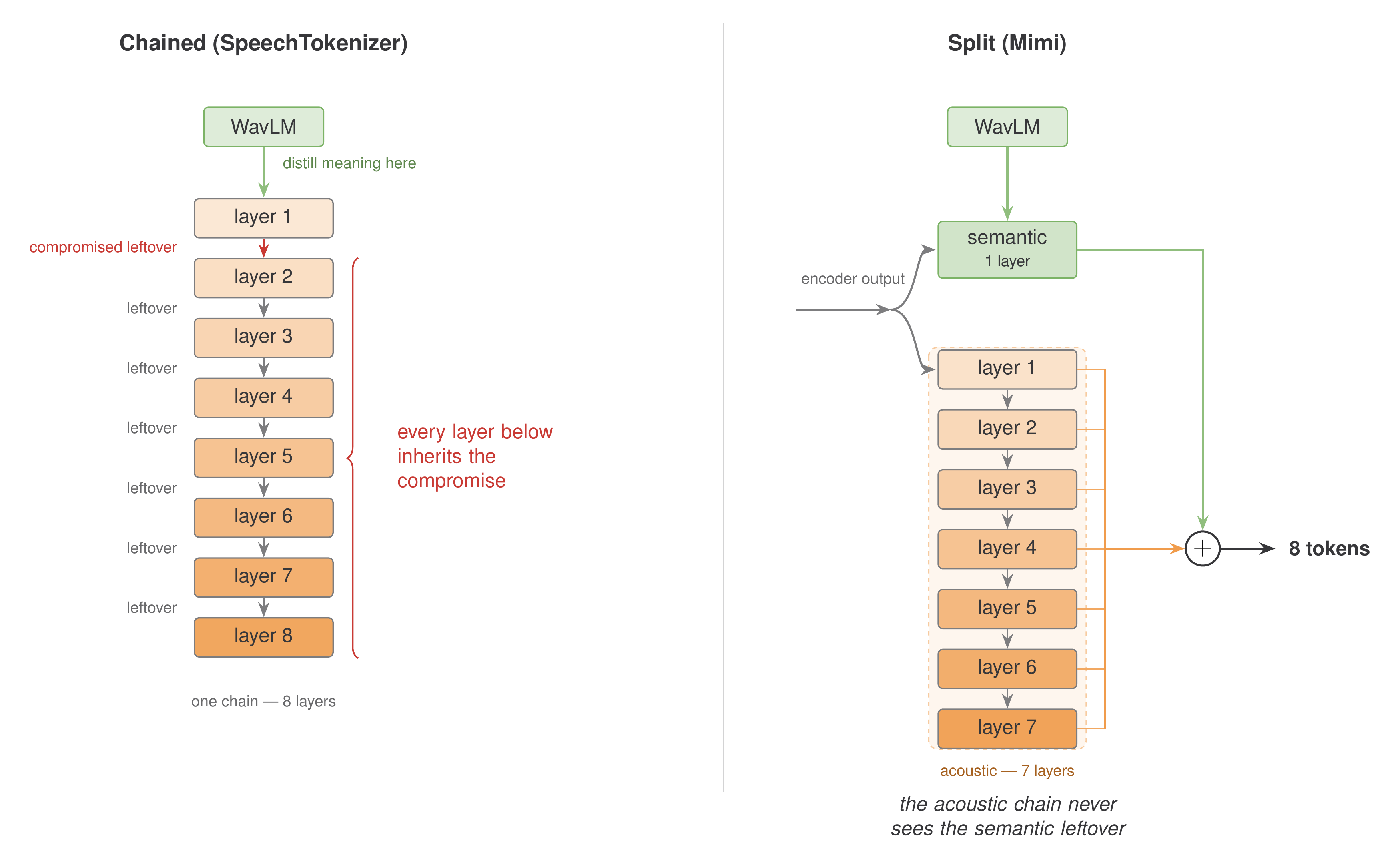
Figure 4 - Why Mimi splits the quantizer. Chaining meaning in front of sound poisons everything below it.

---

Part 8: The text side — putting words on the audio clock

Everything so far handles sound. But Moshi also predicts a text token every frame, its “Inner Monologue” — it writes down what it’s about to say, then says it. This turns out to matter a lot for whether the model talks sense.

It also creates a scheduling problem people underestimate.

Audio runs at 12.5 frames per second. Words arrive at about 3–4 per second. So most frames have no word in them. You can’t just pair them up — there’s nothing to pair.

Moshi’s solution has two parts.

First, find out when each word is actually spoken. Run Whisper over the training audio to get word-level timestamps, so you know that “hello” starts at 1.04 seconds and therefore belongs to frame 13.

Second, invent two filler tokens for the empty frames: PAD for “nothing being said right now,” and EPAD for “padding is about to end, a word is coming.”

The construction is short enough to write out completely:

PAD, EPAD = "<pad>", "<epad>"

def build_text_stream(words, start_times, n_frames, frame_rate=12.5):
    # 1. Start with every frame empty.
    W = [PAD] * n_frames

    # 2. Drop each word in at the frame where it's actually spoken.
    for word_tokens, t in zip(words, start_times):
        f = int(t * frame_rate)                 # seconds -> frame number
        for j, tok in enumerate(word_tokens):
            W[f + j] = tok

    # 3. Put EPAD right before each word: "get ready, one's coming".
    for word_tokens, t in zip(words, start_times):
        f = int(t * frame_rate)
        if f > 0 and W[f - 1] == PAD:
            W[f - 1] = EPAD

    return W

# For "hello ... there":
#   [PAD, PAD, "hel", "lo", PAD, PAD, PAD, EPAD, "there", PAD, ...]

Why bother with EPAD? Because it splits one hard decision into two easy ones. Without it, the model must decide whether to start talking and what word to say in the same step. With it, emitting EPAD answers only “I’m about to speak,” and the next frame answers “here’s the word.”

Which hands you a remarkably direct control knob: force an EPAD into the text stream and the model starts talking immediately. Turn-taking, the thing that took cascaded systems an entire subsystem of voice-activity detection and endpointing heuristics, becomes a one-token intervention.

Two more consequences fall out of this design, and both are elegant.

The text stream only covers Moshi’s own speech, never the user’s. That’s deliberate. Transcribing the user in real time would require an external ASR system — exactly the cascaded architecture the whole approach exists to avoid. Moshi thinks in text about what it is saying, and hears you purely as sound.

Swap the ordering and the same model changes jobs. Put text behind audio and it transcribes what it just heard: streaming ASR. Put text ahead of audio and it speaks what it just read: streaming TTS. Same weights, one changed offset. Speech recognition and speech synthesis turn out to be one model viewed from two directions.

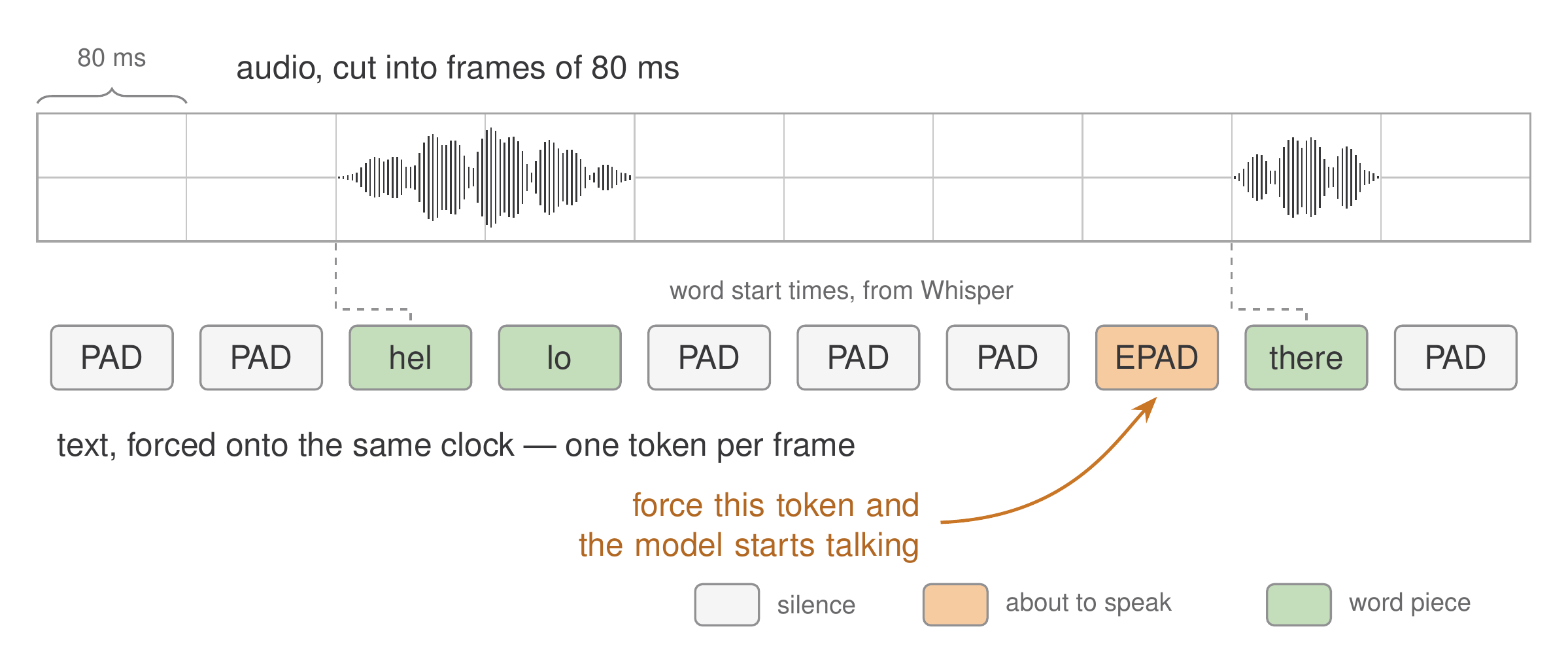
Figure 5 - Words on the audio clock. PAD fills the silence; EPAD announces that a word is coming.

---

Part 9: The round trip

Every piece together — one frame in the life of a full-duplex model:

def one_frame(model, mic_samples, state):
    """80 milliseconds. 1,920 samples in, 1,920 samples out."""

    # --- IN: sound becomes integers ---
    z        = model.mimi.encoder(mic_samples)   # 1,920 samples -> one summary vector
    user_tok = model.mimi.quantizer.encode(z)    # -> 8 integers

    # --- THINK: one step of the language model ---
    h, state = model.temporal.step(state)        # the big model, once per frame
    text_tok = model.depth.predict_text(h)       # PAD / EPAD / a word piece
    own_tok  = model.depth.predict_audio(h, text_tok)   # 8 integers, coarse to fine

    # --- OUT: integers become sound ---
    z_out    = model.mimi.quantizer.decode(own_tok)  # add up the 8 layers
    speaker  = model.mimi.decoder(z_out)             # -> 1,920 samples

    return speaker, text_tok, state

# 12.5 times a second. Forever. Under 80 milliseconds each time.

Seventeen integers per frame — 8 for what it hears, 8 for what it says, 1 for what it’s thinking — is the entire interface between a conversation and a language model.

One small mechanism I’ll mention without belabouring: the acoustic layers are usually shifted one frame later than the semantic layer, so the model has committed to what it’s saying before it fills in how it sounds. That one-frame shift is also, directly, half of Moshi’s 160ms latency budget — 80ms for the frame plus 80ms for the shift. In this field, every design choice eventually shows up as milliseconds.

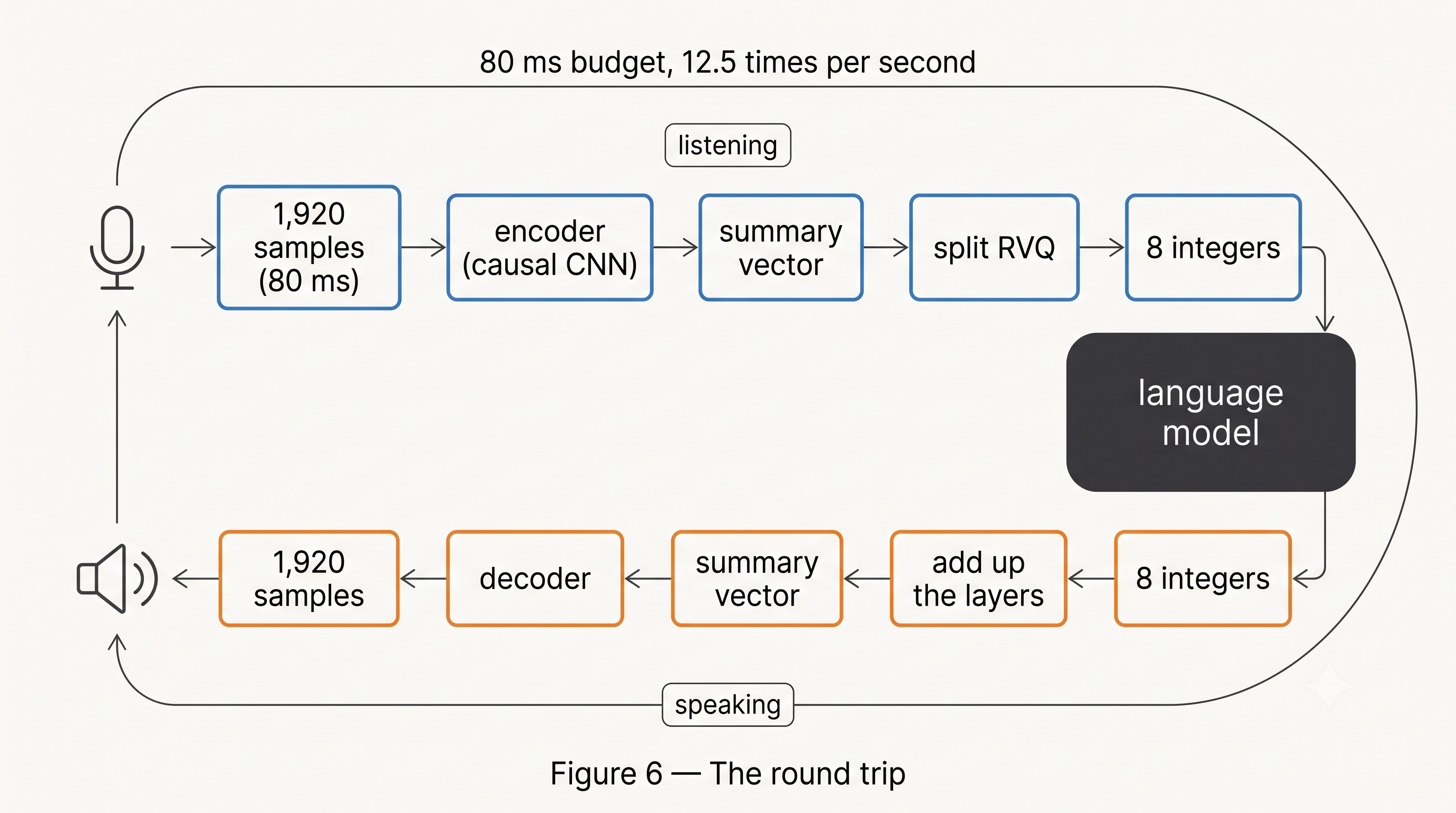
Figure 6 - The round trip. Seventeen integers per frame is the whole interface.

---

Part 10: What’s still hard

The codec is a ceiling. Whatever it discards is gone, permanently, and no amount of scaling the language model brings it back. If Mimi’s 1.1 kbps doesn’t preserve some subtle prosodic cue, no model built on Mimi can ever respond to that cue. Codec design sits quietly upstream of every capability claim in this field, which is a good reason to care about it more than the attention it usually gets.

Meaning and sound still fight. Split RVQ relieves the pressure inside the codec. It doesn’t eliminate the underlying tension, which resurfaces one level up inside the language model’s own parameters — the gradient-conflict problem Lychee-FD diagnosed, which I wrote about in the previous post.

The timestamps are fragile. Inner Monologue needs word-level timing for every training utterance. That’s expensive to produce and vulnerable to compounding alignment errors. It’s arguably also unnatural: FLM-Audio points out that humans plan in a forward-moving internal stream that generally runs ahead of speech, rather than emitting exactly one thought-unit per 80ms tick. Approaches that relax strict alignment are an active area.

Nobody knows the right frame rate. 12.5 Hz was chosen to sit near English text rates. Go lower and sequences get cheaper but reconstruction gets harder; go higher and quality is easier but the language model drowns. There’s no established optimum, and it plausibly differs across languages — a language with a faster syllable rate than English may be poorly served by a number tuned on English.

Evaluation measures the wrong thing. Codec papers report reconstruction quality. But what you actually care about is how good a language model you can train on these tokens, which is a different question with a different answer. SpeechTokenizer’s benchmark was an early attempt to measure it directly. The gap is still wide.

---

The short version

A language model can only consume integers, and audio doesn’t come with any. A neural audio codec invents them: an encoder network summarizes each 80ms of sound into a vector, and vector quantization rounds that vector to the nearest entry in a learned dictionary, yielding an integer.

One dictionary would need about 10²⁶ entries to be expressive enough, so instead we describe sound in layers — a rough guess, then a correction, then a finer correction. Residual vector quantization gets the same expressive range from 16,384 stored vectors instead of 10²⁶, and that’s why any of this works.

Mimi adds three things: a frame rate picked to sit near text token rates, fully causal operation so it streams, and a split quantizer that runs the meaning-carrying layer alongside the sound-carrying ones rather than in front of them — because chaining them made one poison the other. And Inner Monologue puts words onto the same clock using Whisper timestamps plus filler tokens, which as a side effect makes turn-taking a single-token decision and makes speech recognition and speech synthesis the same model read in opposite directions.

---

References

Foundations

1. Dudley, H. (1939). The Vocoder. Bell Labs Record, 17:122–126. The original analysis-synthesis idea.

2. van den Oord, A., Dieleman, S., Zen, H., Simonyan, K., Vinyals, O., Graves, A., Kalchbrenner, N., Senior, A., & Kavukcuoglu, K. (2016). WaveNet: A Generative Model for Raw Audio. arXiv:1609.03499. https://arxiv.org/abs/1609.03499

3. van den Oord, A., Vinyals, O., & Kavukcuoglu, K. (2017). Neural Discrete Representation Learning (VQ-VAE). arXiv:1711.00937. https://arxiv.org/abs/1711.00937

The compression lineage

1. Kleijn, W. B., Lim, F. S. C., Luebs, A., Skoglund, J., Stimberg, F., Wang, Q., & Walters, T. C. (2018). WaveNet Based Low Rate Speech Coding. ICASSP 2018, pp. 676–680. arXiv:1712.01120. https://arxiv.org/abs/1712.01120

2. Gârbacea, C., van den Oord, A., Li, Y., Lim, F. S. C., Luebs, A., Vinyals, O., & Walters, T. C. (2019). Low Bit-rate Speech Coding with VQ-VAE and a WaveNet Decoder. ICASSP 2019.

3. Zeghidour, N., Luebs, A., Omran, A., Skoglund, J., & Tagliasacchi, M. (2021). SoundStream: An End-to-End Neural Audio Codec. IEEE/ACM TASLP, 30:495–507. arXiv:2107.03312. https://arxiv.org/abs/2107.03312

4. Défossez, A., Copet, J., Synnaeve, G., & Adi, Y. (2022). High Fidelity Neural Audio Compression (EnCodec). TMLR 2023. arXiv:2210.13438. https://arxiv.org/abs/2210.13438

5. Kumar, R., Seetharaman, P., Luebs, A., Kumar, I., & Kumar, K. (2023). High-Fidelity Audio Compression with Improved RVQGAN (Descript Audio Codec). NeurIPS 2023. arXiv:2306.06546. https://arxiv.org/abs/2306.06546

The understanding lineage

1. Baevski, A., Zhou, H., Mohamed, A., & Auli, M. (2020). wav2vec 2.0: A Framework for Self-Supervised Learning of Speech Representations. arXiv:2006.11477. https://arxiv.org/abs/2006.11477

2. Hsu, W.-N., Bolte, B., Tsai, Y.-H. H., Lakhotia, K., Salakhutdinov, R., & Mohamed, A. (2021). HuBERT: Self-Supervised Speech Representation Learning by Masked Prediction of Hidden Units. arXiv:2106.07447. https://arxiv.org/abs/2106.07447

3. Chen, S., Wang, C., Chen, Z., Wu, Y., Liu, S., Chen, Z., Li, J., Kanda, N., Yoshioka, T., Xiao, X., et al. (2022). WavLM: Large-Scale Self-Supervised Pre-Training for Full Stack Speech Processing. IEEE JSTSP. arXiv:2110.13900. https://arxiv.org/abs/2110.13900

The merge

1. Borsos, Z., Marinier, R., Vincent, D., Kharitonov, E., Pietquin, O., Sharifi, M., Roblek, D., Teboul, O., Grangier, D., Tagliasacchi, M., & Zeghidour, N. (2022). AudioLM: a Language Modeling Approach to Audio Generation. arXiv:2209.03143. https://arxiv.org/abs/2209.03143

2. Zhang, X., Zhang, D., Li, S., Zhou, Y., & Qiu, X. (2024). SpeechTokenizer: Unified Speech Tokenizer for Speech Large Language Models. ICLR 2024. arXiv:2308.16692. https://arxiv.org/abs/2308.16692

3. Défossez, A., Mazaré, L., Orsini, M., Royer, A., Pérez, P., Jégou, H., Grave, E., & Zeghidour, N. (2024). Moshi: a speech-text foundation model for real-time dialogue. arXiv:2410.00037. https://arxiv.org/abs/2410.00037 · Code: https://github.com/kyutai-labs/moshi · Weights: https://huggingface.co/kyutai/mimi · Accessible explainer: https://kyutai.org/codec-explainer

Supporting

1. Copet, J., Kreuk, F., Gat, I., Remez, T., Kant, D., Synnaeve, G., Adi, Y., & Défossez, A. (2023). Simple and Controllable Music Generation (MusicGen). NeurIPS 2023. arXiv:2306.05284. https://arxiv.org/abs/2306.05284 — origin of the codebook delay patterns.

2. Radford, A., Kim, J. W., Xu, T., Brockman, G., McLeavey, C., & Sutskever, I. (2022). Robust Speech Recognition via Large-Scale Weak Supervision (Whisper). arXiv:2212.04356. https://arxiv.org/abs/2212.04356

3. FLM-Audio: Natural Monologues Improve Native Full-Duplex Chatbots via Dual Training. (2025). arXiv:2509.02521. https://arxiv.org/abs/2509.02521 — critiques strict token-level text/audio alignment.

---

*Code snippets are illustrative pseudocode written to expose the mechanism — they are not runnable implementations. For working code, see the linked repositories.